How Did Google Researchers Beat ImageNet While Using Fewer Resources?
Did they invent a new model? Read on…
Hey, it’s Devansh 👋👋
In my series Breakdowns, I go through complicated literature on Machine Learning to extract the most valuable insights. Expect concise, jargon-free, but still useful analysis aimed at helping you understand the intricacies of Cutting Edge AI Research and the applications of Deep Learning at the highest level.
If you’d like to support my writing, please consider buying and rating my 1 Dollar Ebook on Amazon or becoming a premium subscriber to my sister publication Tech Made Simple using the button below.
p.s. you can learn more about the paid plan here.
Image Classification algorithms have been getting better mostly by using more resources (data, computing power, and time). The best algorithms use an extra 3.5 Billion labelled images. This paper, written by Qizhe Xie et al bucks the trend. It is able to beat the current algorithms while using only an extra 300 M unlabeled images (both algorithms use the same labelled Dataset of images, on which we have the extra 3.5 B and 300 M images respectively). This means that the new method uses 12 times lesser images, while also not requiring those images to be labelled. Therefore it is many, many times cheaper while giving better results.
What does this team do differently?
To understand this paper and the experiment set-up check out this video.
On the surface, their approach seems to be standard SSL. The key to their superior performance lies in the steps taken before and during training. The unlabeled student model is larger than the teacher. The team also injects different types of noise into the data and models, ensuring that each student learns on more types of data distributions than their teachers. This combined with the Iterative Training is especially powerful since this makes use of the constantly improving teachers.
All about that noise
Since we have established the importance of noise in this training, it is important to understand the different kinds of noise involved. There are two broad categories of noise that can be implemented. Model noise refers to messing with the model during the training process. This prevents overfitting and might actually boost accuracy and robustness by allowing the model to evaluate the data with different “perspectives”. The other kind is called input noise where you inject noise to the input. The researchers specifically use RandAugment to achieve this. This serves a dual purpose of increasing the variety of data, and improving the accuracy of predictions (especially for real-world data, which is very noisy).
Exhibit 1: RandAugment for Input Noise
There are some really complicated noise functions in the world. RandAugment is not one of them. Don’t be fooled though, it is one of the most effective algorithms out there. It works in a really easy to understand way. Imagine there are N ways to distort an image. This can be anything, from changing some pixels to white, to shearing along an axis. RandAugment takes 2 inputs (n,m) where n is the number of distortions applied and m is the magnitude of the distortions. It returns the final image. The distortions are applied randomly, increasing the noise by adding variability.
In the image, we see RandAugment at work applying only 2 (fixed) transformations at varying magnitudes. Already these 3 samples are very different. It doesn’t take a genius to figure out how many you could get by varying both values across multiple images (answer: lots). The data augmentation should not be overlooked. It also ensures that the student model is always at least as big as the teacher, and therefore requires fewer
Exhibit 2: Dropout for Model Noise
Dropout is a process used on neural networks etc. Its process is very easy to describe: ignore some neurons every run of the network. Pictorially:
Dropout is applied because it stops overfitting. By ignoring different units, you change the output. The feedback allows it to generalize better. Additionally, dropout can be implemented to create a list of mini-learners from one network. By ensembling, the mini-learners can outperform the parent network.
Exhibit 3: Stochastic Depth for Model Noise
Tobe frank, I wasn’t super familiar with this concept. But hey that’s what Google is for. Reading into this was amazing. Probably my favorite thing this whole paper. If I had to restart life with only one memory, this would be it. Now that we have built up the hype…
Stochastic Depth involves the following steps.
Start with very deep networks
During training, for each mini-batch, randomly drop a subset of layers and bypass them with the identity function.
Repeat (if needed)
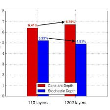
This seems awfully similar to Dropout. And in a way it is. Think of it as a scaled-up version for deep networks. However, it is really effective. “ It reduces training time substantially and improves the test error significantly on almost all data sets that we used for evaluation. With stochastic depth we can increase the depth of residual networks even beyond 1200 layers and still yield meaningful improvements in test error (4.91 % on CIFAR-10).” Can’t argue with that. Will be delving into this soon. For now, look at this figure plotting error:
The 3 Kinds of Noise all contribute to the training in a unique way. And all 3 are amazing for adding robustness to predictions, by adding variation to input. This is what sets it apart in robustness from all the other State of the Art models. They are in fact so effective that even without the iterative training process, the process is able to improve current state of the art networks (more details on this in Pt 2).
Training Process
Now that we understand how the different steps and adjustments improve the classification, we should look into some of the implementation details.
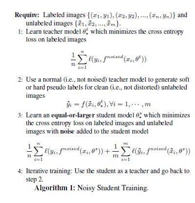
To me, the most significant part of the training comes in step 3. The researchers state that “Specifically, in our method, the teacher produces high-quality pseudo labels by reading in clean images, while the student is required to reproduce those labels with augmented images as input.” As we have seen, adding noise to the images (or models) can drastically change how they look. By forcing the student to work with augmented images, it allows the model to predict very unclear images with great accuracy. The details of this will be in Pt 2. but for now, here’s an example of how crucial this is in predicting ambiguous images.
For Machine Learning a base in Software Engineering, Math, and Computer Science is crucial. It will help you conceptualize, build, and optimize your ML. My daily newsletter, Technology Made Simple covers topics in Algorithm Design, Math, Recent Events in Tech, Software Engineering, and much more to make you a better Machine Learning Engineer. I have a special discount for my readers.
Save the time, energy, and money you would burn by going through all those videos, courses, products, and ‘coaches’ and easily find all your needs met in one place.
I am currently running a 20% discount for a WHOLE YEAR, so make sure to check it out. Using this discount will drop the prices-
800 INR (10 USD) → 533 INR (8 USD) per Month
8000 INR (100 USD) → 6400INR (80 USD) per year
You can learn more about the newsletter here. If you’d like to talk to me about your project/company/organization, scroll below and use my contact links to reach out to me.
Reach out to me
Use the links below to check out my other content, learn more about tutoring, reach out to me about projects, or just to say hi.
If you like my writing, I would really appreciate an anonymous testimonial. You can drop it here.
To help me understand you fill out this survey (anonymous)
Check out my other articles on Medium. : https://rb.gy/zn1aiu
My YouTube: https://rb.gy/88iwdd
Reach out to me on LinkedIn. Let’s connect: https://rb.gy/m5ok2y
My Instagram: https://rb.gy/gmvuy9
My Twitter: https://twitter.com/Machine01776819


M
V. C.
No p
P
‘
Z j no
B. I.
, B. lol o
Cc.