I came across an interesting Paper named, “Deep Ensembles: A Loss Landscape Perspective” by a Laxshminarayan et al. In this article, I will break down the paper, summarise its findings and delve into some of the techniques and strategies they used that will be useful for delving into understanding models and their learning process. It will also go over some possible extensions to the paper.
If you’re busy, here’s a quick video. It explains the crux of the paper, including the hypothesis and conclusion of the paper. Feel free to check it out instead. This article will go into more detail and watching the video is not necessary to understand the article. Any feedback on the video would be much appreciated though. Don’t forget to like and sub :)
The Theory
The authors conjectured (correctly) that Deep Ensembles (an ensemble of Deep learning models) outperform Bayesian Neural Networks because “popular scalable variational Bayesian methods tend to focus on a single mode, whereas deep ensembles tend to explore diverse modes in function space.”
In simple words, when running a Bayesian Network at a single initialization it will reach one of the peaks and stop. Deep ensembles will explore different modes, therefore reducing error when put in practice. In picture form:
Depending on it’s hyperparameters, a single run of a bayesian network will find one of the paths (colors)and it’s mode. Therefore it won’t explore the set of parameters. On the other hand, a deep ensemble will explore all the paths, and therefore get a better understanding of the weight space (and solutions). To understand why this translates to better understanding consider the following illustration.
In the diagram, we have 3 possible solution spaces, corresponding to each of the trajectories. The optimized mode for each gives a performance gives us a score of 90% (for example). Each mode is unable to solve a certain kind of problem (highlighted in red). A Bayesian Network will get to either A, B, or C in a run while a Deep Ensemble will be able to train over all 3.
The Techniques
They proved their hypothesis using various strategies. This allowed them to approach the problem from various perspectives. I will show the details for each of them.
Cosine Similarity:
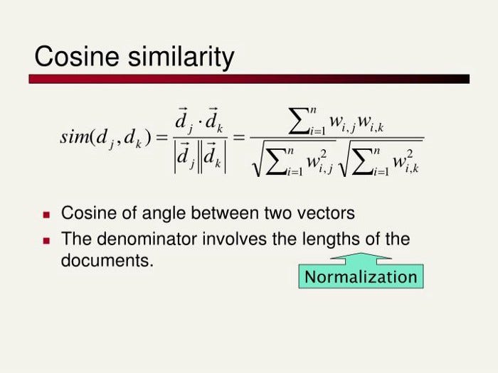
Cosine similarity is defined, as the “measure of similarity between two non-zero vectors of an inner product space. It is defined to equal the cosine of the angle between them, which is also the same as the inner product of the same vectors normalized to both have length 1.” It is derived from the dot product between vectors. Imagine 3 texts: A, B, and C. A and C and large documents on a similar topic and B is a very short summary of A. A and C might end up having a low Euclidean Distance because they have a lot of overlapping words or phrases, while A and B will have a larger distance because of the difference in size. The cosine similarities would paint a different picture, however, since A and B would have a low angle (thus high similarity) between them.
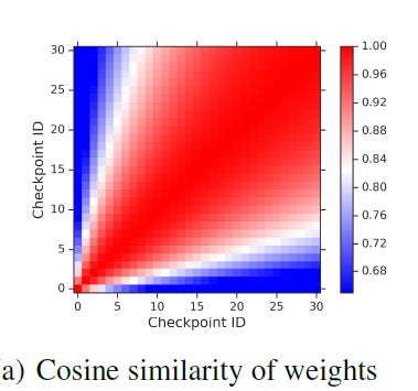
This diagram is used to show that “checkpoints along a trajectory are largely similar both in the weight space and the function space.” Checkpoint 30 and Checkpoint 25 have high similarity (red) while 30 and 5 have relatively low similarity (grey). An interesting thing to note is that the lowest labeled point is a similarity of 0.68. This goes to show how quickly models
Disagreement in Function Space:
Defined as “the fraction of points the checkpoints disagree on”, or,
network for input x:
Disagreement is like the complement to the similarity scores and serves to showcase the difference in checkpoints along the same trajectory in a more direct manner. Both similarity and disagreement are calculated over a single run with a single model. The highest slab for disagreement starts at 0.45. This shows that there is relatively low disagreement, consistent with the findings of the similarity map.
The use of disagreement and similarity shows that points along the same trajectory have very similar predictions. The third way is used to prove that trajectories can take very different paths, and thus end up unable to solve certain kinds of problems.
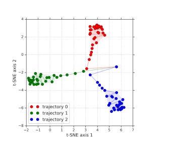
Plotting Different Random Initializations using tsne
As stated before, this diagram is used to show how different random initializations differ in function space. It is used to effectively plot the higher dimensional data into lower (human understandable) dimensions. It is an alternative to PCA. Unlike PCA, tSNE is non-linear and probabilistic in nature. It is also far more computationally expensive (esp. with lots of samples and high dimensionality). In this context, TSNE makes more sense than PCA because deep learning is also not a linear process, so TSNE suits it better. The researchers applied some preprocessing to keep the costs down. The steps they took specifically were, “for each checkpoint we take the softmax output for a set of examples, flatten the vector and use it to represent the model’s predictions. The t-SNE algorithm is then used to reduce it to a 2D point in the t-SNE plot. Figure 2(c) shows that the functions explored by different trajectories (denoted by circles with different colors) are far away, while functions explored within a single trajectory (circles with the same color) tend to be much more similar.”
Subspace Sampling and Diversity Measurement
The last 2 things the paper implemented were subspace sampling and diversity measurement. Subspace sampling involves training the data without all the features. This can be used to create several learners, that when combined, perform better than the original. The details of the sampling methods are in the paper. The samples, validated the results of the full-feature tsne, with random initializations going along different paths.
The diversity score quantifies the difference of two functions (a base solution and a sampled one), by measuring the fraction of data points on which the predictions differ. This simple approach is enough to validate the premise
Both the sampling and accuracy-diversity plots are further proof of the hypothesis.
Combined these techniques prove two things:
Different initializations of a network will cause a model to reach and get stuck at different modes (peaks). This will let it solve certain problems and not others. Points along the trajectory along to the mode will have very similar predictions.
Ensembles are able to learn from multiple modes, thus improve their performance.
Extensions
This paper was great in popping the hood behind the learning processes Deep Ensembles and Bayesian Networks. An analysis of the learning curves and validation curves would’ve been interesting. Furthermore, it would be interesting to see how deep learning ensembles stack up Random Forests, or other ensembles. Performing a similar analysis on the learning processes of these would allow us to create mixed ensembles that might use be good for solving complex problems.
For Machine Learning a base in Software Engineering, Math, and Computer Science is crucial. It will help you conceptualize, build, and optimize your ML. My daily newsletter, Technology Made Simple covers topics in Algorithm Design, Math, Recent Events in Tech, Software Engineering, and much more to make you a better Machine Learning Engineer. I have a special discount for my readers.
Save the time, energy, and money you would burn by going through all those videos, courses, products, and ‘coaches’ and easily find all your needs met in one place.
I am currently running a 20% discount for a WHOLE YEAR, so make sure to check it out. Using this discount will drop the prices-
800 INR (10 USD) → 533 INR (8 USD) per Month
8000 INR (100 USD) → 6400INR (80 USD) per year
You can learn more about the newsletter here. If you’d like to talk to me about your project/company/organization, scroll below and use my contact links to reach out to me.
Reach out to me
Use the links below to check out my other content, learn more about tutoring, reach out to me about projects, or just to say hi.
If you like my writing, I would really appreciate an anonymous testimonial. You can drop it here.
To help me understand you fill out this survey (anonymous)
Check out my other articles on Medium. : https://rb.gy/zn1aiu
My YouTube: https://rb.gy/88iwdd
Reach out to me on LinkedIn. Let’s connect: https://rb.gy/m5ok2y
My Instagram: https://rb.gy/gmvuy9
My Twitter: https://twitter.com/Machine01776819
If you’re looking to build a career in tech:


