
How Google and Stanford made AI more Interpretable with a 20 year old Technique [Breakdowns]
An Interpretable Alternative to AutoEncoders. Breaking down: "DB-KSVD: Scalable Alternating Optimization for Disentangling High-Dimensional Embedding Spaces"

It takes time to create work that’s clear, independent, and genuinely useful. If you’ve found value in this newsletter, consider becoming a paid subscriber. It helps me dive deeper into research, reach more people, stay free from ads/hidden agendas, and supports my crippling chocolate milk addiction. We run on a “pay what you can” model—so if you believe in the mission, there’s likely a plan that fits (over here).
Every subscription helps me stay independent, avoid clickbait, and focus on depth over noise, and I deeply appreciate everyone who chooses to support our cult.
PS – Supporting this work doesn’t have to come out of your pocket. If you read this as part of your professional development, you can use this email template to request reimbursement for your subscription.
Every month, the Chocolate Milk Cult reaches over a million Builders, Investors, Policy Makers, Leaders, and more. If you’d like to meet other members of our community, please fill out this contact form here (I will never sell your data nor will I make intros w/o your explicit permission)- https://forms.gle/Pi1pGLuS1FmzXoLr6
Interpretability research is one of the most underpriced elements in AI right now. As multiple contenders vie for AI supremacy, a key deciding factor in adoption will be the trustworthiness of AI systems in high-value fields like medicine, law, finance, insurance, and more. As we’ve noted in prior articles, market dynamics have consistently overpriced base model intelligence while underpricing model reliability and deployment readiness.
Some of this is pragmatic — investors seek predictable returns after seeing many vaporware startups collapse, and AGI remains a magnet word in the market. But with inflated valuations, endless copycats, and rising AI fatigue, this is the moment to explore new directions that can expand markets.
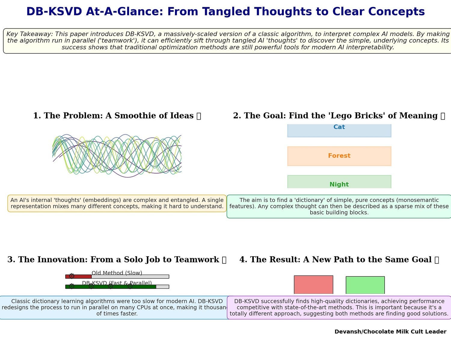
Interpretability research itself has reached an inflection point. Sparse autoencoders (SAEs) have dominated recent years as the scalable tool for disentangling embeddings. They became the benchmark, the default probe. But new work on DB-KSVD, a re-engineered classic algorithm, shows that SAEs are not unique in their performance —
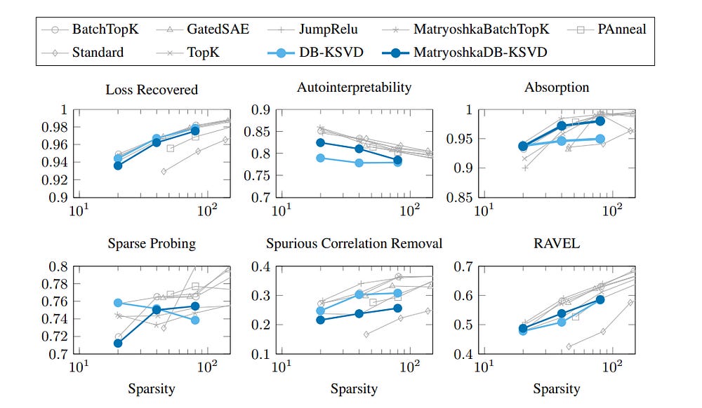
“We demonstrate the efficacy of DB-KSVD by disentangling embeddings of the Gemma-2–2B model and evaluating on six metrics from the SAEBench benchmark, where we achieve competitive results when compared to established approaches based on SAEs. By matching SAE performance with an entirely different optimization approach, our results suggest that (i) SAEs do find strong solutions to the dictionary learning problem and (ii) that traditional optimization approaches can be scaled to the required problem sizes, offering a promising avenue for further research.” (This amazing performance is what interested me first, given it’s implications for more interpretable legal AI for our work at Iqidis)

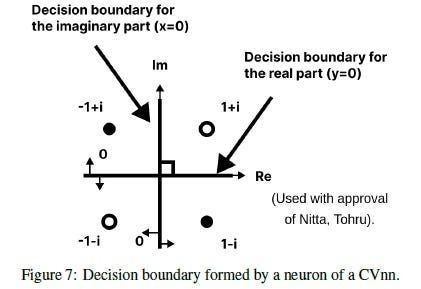
This similarity in performance is a larger signal than it seems. Two very different approaches now converge on the same ceiling. The convergence of these opposite approaches signals that the boundary is not in the optimizer, but in the geometry of high-dimensional spaces (an idea we also saw with Natural Gradients, Kimi, and Complex Valued Neural Networks). If we want to push further, the next frontier will require new mathematics and new hardware (more on this both in this article and in a detailed market report on interpretable AI).
This article will deconstruct this convergence from first principles. We will:
Detail the mechanisms of both SAEs and the K-SVD algorithm.
Analyze why two fundamentally different methods arrived at the same performance ceiling.
Break down the geometric (algorithmic/mathematical) and physical (in our current hardware/how we handle memory) limits that this reveals convergence.
Extrapolate how this research/the ideas discussed impact the future of AI hardware and the next generation of interpretability research.
This article was a pain to research and put together, and I can’t imagine it will be a cakewalk to read. We’ll blend exhaustive discussions of math, computer science, and classical AI techniques within a larger frame of geopolitical and macroeconomic pressures. We’re digging deep into the algorithms b/c it’s the only way for us to appreciate the profound implications of what this research hints at (and how we can build on it). Y’all got big brains, so I won’t be coddling you w/ oversimplifications or skipped details. I trust you’ll find a way to keep up. The importance of the ideas discussed merit the investment.
PS- If, despite your best efforts, you have trouble understanding this, send me flight tickets and accommodation fees, and I’ll show up at your doorstep in my best teacher outfit for some personal tutoring. My rates aren’t cheap though :))
Executive Highlights (TL;DR of the Article)
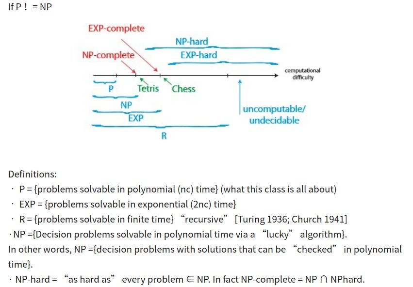
To interpret and trust AI models, we must deconstruct their internal representations — a process known as dictionary learning, mathematically formulated as Y ≈ DX. This task is NP-hard. For years, the field has relied on Sparse Autoencoders (SAEs), a scalable but heuristic neural network approach, leaving open the question of whether their solutions reflect ground truth.
A recent paper re-engineered a classic, deterministic algorithm (K-SVD) to operate at a modern scale (DB-KSVD). When benchmarked against state-of-the-art SAEs, it achieved nearly identical performance. The convergence of these two philosophically opposite methods — one a gradient-based heuristic, the other an iterative, structured optimizer — hints that the performance ceiling is not a flaw in our algorithms but a fundamental limit of the problem itself.
This problem comes from the limits of geometry of linear spaces and their limitations. This discovery has two direct and unavoidable consequences for the future of AI:
The Mathematical Frontier is Now Non-Linear: Since our best linear tools have hit a hard ceiling, the next breakthroughs in interpretability must come from non-linear mathematics. The field must now move towards tools like manifold learning and kernel methods to capture the true, likely curved, geometry of the model’s internal representations.
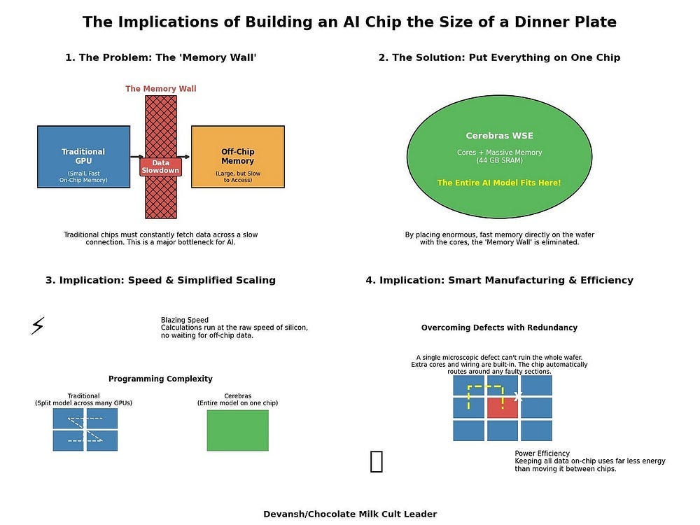
The Physical Frontier is the Memory Wall: The engineering required to scale K-SVD (trading computation for memory) highlights that our ability to perform sophisticated AI analysis is physically constrained by memory bandwidth. This creates a direct economic incentive for new, memory-centric hardware (PIM, advanced HBM) designed specifically for the task of AI interpretation and alignment, not just training.
Overall, this space opens up a lot of opportunities across research, investing in interpretable (and thus safe) AI, and w/ how all of this plays against the trends in Hardware. While we will have the deep dive in the follow-up article on the market size for Interpretable AI, there are a few factors that we must be aware of right now —
Geopolitical tensions have everyone looking at their supply chains. Hardware is a strategic resource, and there are massive investments being made to bring manufacturing domestically. This opens up some of the market for specialized chips (since the new factories can accommodate them w/o sinking money into rebuilds).
AI Fatigue is very real, and many people are looking for excuses to avoid adopting AI. Research like this can stop that.
Further developments in adopting AI (and subsequent mishaps) will turn the incumbents' multi-billion-dollar models into assets with a quantifiable, uncorrectable liability. This irreducible ambiguity is a balance sheet risk that prohibits them from signing enterprise SLAs with meaningful guarantees, capping their TAM. The way around here is to invest in interpretability tech.
Regulatory pressure for XAI is strong and will continue to grow due to both political and economic reasons.
As we will discuss, this work piggybacks off the trend of higher memory workloads, making the marginal cost of usage lower.
All of these will put a strong upward pressure on this field of research. This paper is a great signal of a trend that will pick up steam in early 2026, and getting ahead of the space now is best.

Investors pay attention — If the memory wall interests you, an amazing founder I know is raising seed capital for his new startup. The space has a ton of potential, and this founder has in the space for 20 years and was previously part of a 1 billion USD IPO. If you want an introduction email me — devansh@svam.com with information about your fund and thesis. The startup has amazing results — “~30× reduction in footprint, training frontier-scale models in weeks instead of months, running inference at unprecedented speeds by improving model FLOP utilization, and much more”.
Want regular introductions to elite founders and talent? Sign up for a Founding Membership here and reach out to me w/ information on who you’d like to meet.
I put a lot of work into writing this newsletter. To do so, I rely on you for support. If a few more people choose to become paid subscribers, the Chocolate Milk Cult can continue to provide high-quality and accessible education and opportunities to anyone who needs it. If you think this mission is worth contributing to, please consider a premium subscription. You can do so for less than the cost of a Netflix Subscription (pay what you want here).
I provide various consulting and advisory services. If you‘d like to explore how we can work together, reach out to me through any of my socials over here or reply to this email.
Section 1: How Language Models use Geometry to Think
Every modern AI system encodes knowledge by embedding concepts — words, tokens, or higher-order abstractions — into vectors. Each vector is a point in a high-dimensional space. Distances and angles between these points define the semantic structure of the model’s world: words that are closer are considered related, directions correspond to relationships, and clusters capture categories. The angle between the vectors for “king” and “queen” mirrors the angle between “man” and “woman.” This is how models “reason.”
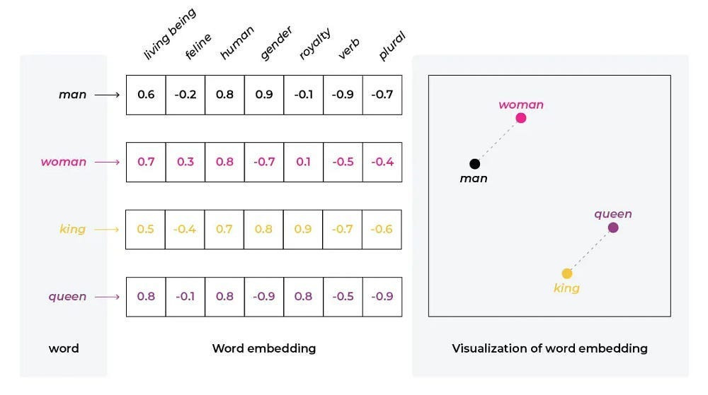
But this space is not cleanly partitioned. For efficiency, models layer thousands of different features into the same vector. This is superposition: a single coordinate encodes multiple, overlapping meanings. Superposition is the reason embeddings are so powerful, but also why they are so opaque. The representation is dense and information-rich, but for humans, almost unreadable.
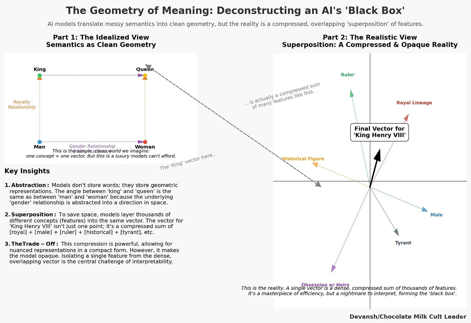
To make AI safe, to underwrite its decisions, to trust it with anything that matters, we must reverse this process. We have to break the superposition. We must find the “atomic basis” — the dictionary of pure, monosemantic features — that the model uses to construct its world.
This brings us to the central equation of modern interpretability research:
Y ≈ DX
This equation is the only path out of the black box. Let’s understand each term:
Y is the data: a matrix where each column is a messy, superimposed embedding vector from the model. Our goal is to reconstruct it.
D is the dictionary: the set of pure, monosemantic features. Each column is a clean vector — “[male],” “[ruler],” or “[obsession with heirs]” — isolated from the rest.
X is the sparse code: the recipe for reconstructing each embedding from a few features in D. Sparsity (mostly zeros) is essential; it enforces the idea that any concept is built from a handful of fundamentals, not thousands.
The entire field, from academic labs to the safety teams at top AI companies, is dedicated to solving this equation. For years, one approach has dominated. That dominance is now challenged — and what’s revealed is not which algorithm is better, but the ceiling they both share.
Section 2: Why We Started Using Sparse Autoencoders
The problem of solving Y ≈ DX is notoriously difficult. Finding the optimal dictionary D and sparse codes X is NP-hard, meaning no known algorithm can solve it efficiently as the problem size grows. In the face of this computational cliff, the AI research community did what so many of us do best: settled for good enough. In this case, this came from a heuristic.
This heuristic is the Sparse Autoencoder (SAE). For the past several years, it has been the undisputed tool of choice for disentanglement. Its design is simple and elegant:
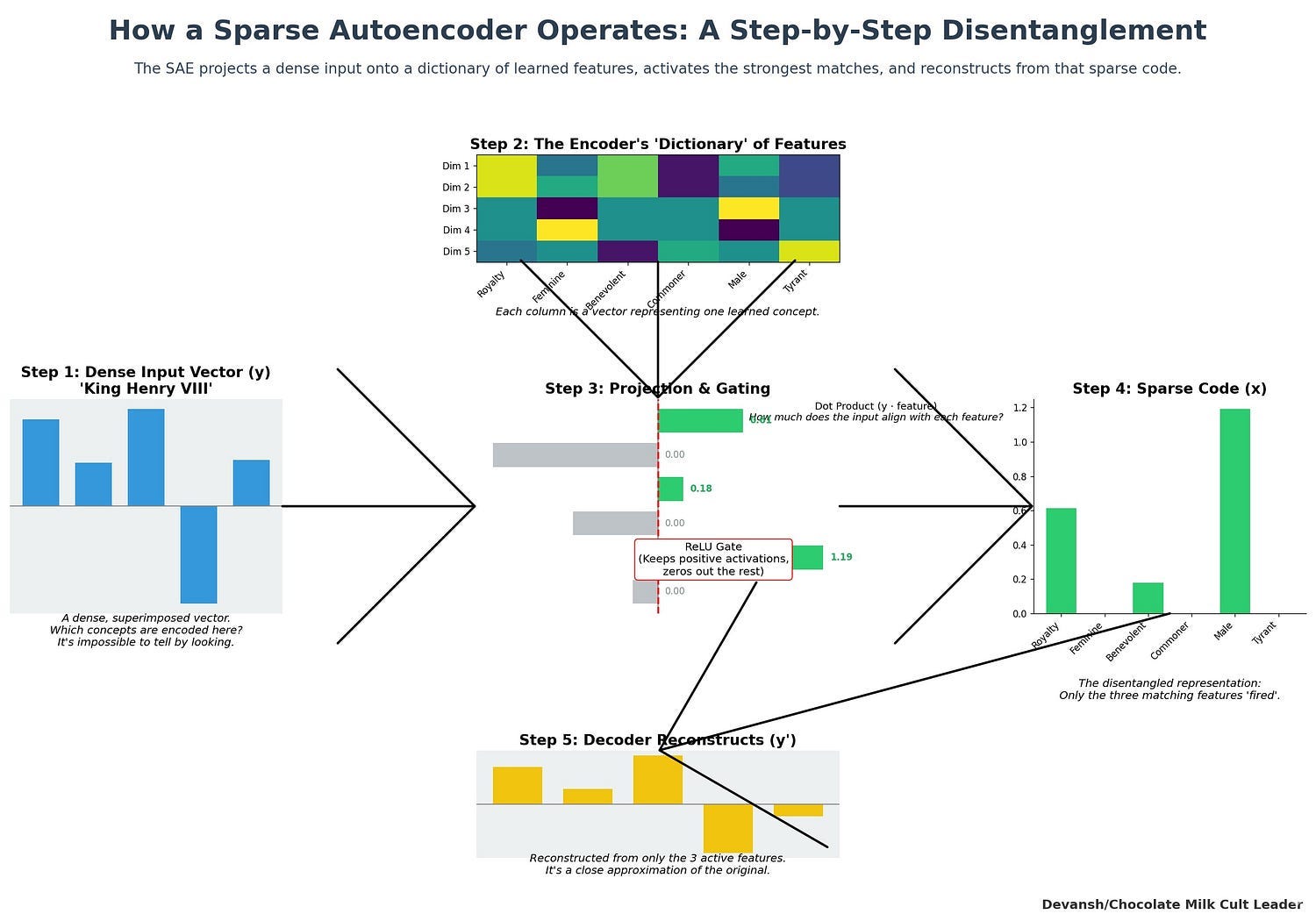
An Encoder: A linear layer followed by a non-linear activation function (like ReLU). The encoder takes dense, superimposed embedding y and transforms it into a high-dimensional, sparse vector x. The weights of this linear layer effectively become our dictionary, D.
A Decoder: A single linear layer that takes the sparse vector x and attempts to reconstruct the original embedding y.
The entire network is trained end-to-end with gradient descent. The training process is a balancing act, governed by a loss function with two competing terms:
Reconstruction Loss (L2 Norm): This term penalizes the network for differences between the original embedding and the reconstructed one. It pushes the SAE to create a dictionary that can accurately rebuild the input signal.
Sparsity Loss (L1 Norm): This term penalizes the encoder for producing codes x that have too many non-zero values. It forces the network to find recipes that use the fewest possible dictionary features.
SAEs became the default because they work at scale. They leverage the modern deep learning stack — GPUs, automatic differentiation, massive datasets — to find good-enough solutions to an otherwise intractable problem. But this pragmatic success has always been shadowed by a critical, unanswered question.
How Legit are they? You see, SAEs are not principled in the strict sense. They do not solve the dictionary learning problem exactly; they approximate it. The encoder is restricted to a simple linear map, which is unlikely to capture the true optimal sparse assignment in high dimensions. The decoder is optimized to minimize reconstruction error, but there is no guarantee that the features it discovers are unique or even interpretable in a strict mathematical sense. The method works because the heuristics are good enough at scale, not because they guarantee the right solution.
This is the core critique. SAEs have given us practical traction on interpretability, but they leave open the question of whether their features are genuine discoveries or artifacts of the optimization process. Until recently, we lacked a way to test this. But that changes now (or a few months ago, I wanted to run some experiments before making this post).
Section 3: K-SVD, an Alternative to SAEs
Sparse autoencoders give us a heuristic path into interpretability, but they don’t actually solve the dictionary learning problem. K-SVD does. It was created in signal processing and works by alternating optimization: instead of trying to solve everything at once, it breaks the problem into two parts and refines them in turn.
The target is always the same equation:
Y ≈ D × X
Y is the data matrix: all the embedding vectors pulled from a model’s layers. Each column of Y is one embedding.
D is the dictionary: the set of features we want to discover. Each column of D is called a dictionary atom — think of it as one candidate basis vector. The hope is that each atom corresponds to a single, monosemantic feature.
X is the coefficient matrix: the sparse codes. Each column of X shows which atoms are active for a given embedding, and how strongly.
The goal: each embedding y should be explained as a sparse combination of a few atoms from D. In other words, y ≈ D × x, where most entries of x are zero.
Step 1: Sparse Encoding (solving for X given D)
With D fixed, we find the best sparse code x for each embedding y. This is the sparse encoding step.
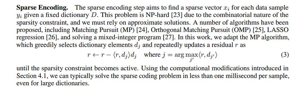
Start with the residual r = y. This is the part of the embedding we still need to explain.
Find the atom d_j most correlated with the residual (the one that has the largest inner product with r).
Add that atom to the code x with the appropriate weight.
Subtract its contribution: update the residual r = r — (weight × d_j). Now r only contains what’s left unexplained.
Repeat until you’ve added at most k atoms. Here k is the sparsity limit: the maximum number of features allowed to explain one embedding.
This process is called Matching Pursuit. It’s greedy and approximate, but fast. The intuition: keep chipping away at the embedding until what’s left is small enough, using only a handful of dictionary atoms.
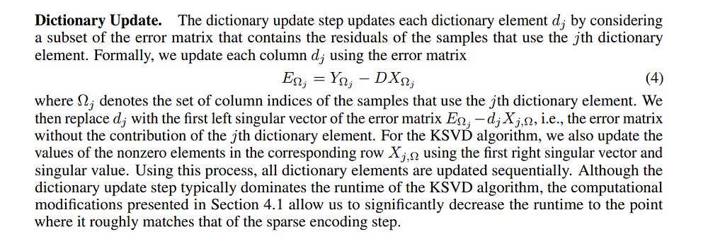
Step 2: Dictionary Update (solving for D given X)
Once the codes X are fixed, we refine the dictionary atoms one by one. For each atom d_j:
Identify all embeddings that actually used d_j in their code (those with a nonzero coefficient in row j of X).
For these embeddings, compute the error you would get if you removed d_j’s contribution. This gives a residual matrix that isolates what d_j is responsible for.
Find the single vector that best explains this residual. K-SVD does this using Singular Value Decomposition (SVD): the top singular vector becomes the new atom d_j.
Update the coefficients for d_j in X based on the corresponding singular values.
This step is surgical: it makes each dictionary atom optimally represent the part of the data that depends on it.
Why K-SVD Mattered and Why It Failed
K-SVD is rigorous. Every step has a clear mathematical role:
Encoding assigns each embedding to a few atoms.
Updating makes each atom specialize to the data that actually uses it.
The problem has always been cost. Sparse encoding requires repeated correlation checks; dictionary updates require repeated SVDs. For small problems (like image patches in denoising or compression), this was fine. For large-scale embeddings — millions of vectors, thousands of dimensions — it was impossible.
So K-SVD suffered the same fate as your wonderful, but needy ex: they were left for someone that’s perhaps not as loving, but is much easier to deal with.
Turns out ex did some therapy, b/c it’s back with a whole new vibe.
4. How DB-KSVD makes K-SVD 10,000x times faster (yes, 10 Thousand Times faster).
The theoretical elegance of K-SVD was never in doubt. Its failure was mechanical: it was too slow for the demands of modern AI. The central achievement of the DB-K-SVD paper is not a new theory, but a feat of algorithmic and systems engineering that bridges this gap. By dissecting K-SVD’s bottlenecks and dismantling them step by step, the authors turned a dormant algorithm into a competitive tool. The process unfolded in three stages.
Part A: The Scaling Breakthrough
The primary drag on K-SVD’s runtime was the sparse encoding step — specifically, the greedy search for the most correlated dictionary atom for each embedding. Doing this iteratively for millions of samples was prohibitive.
The key insight was a space-for-time trade-off. Instead of recomputing correlations from scratch, DB-K-SVD precomputes two massive matrices at the start of each iteration:
DᵀD (m×m): all pairwise inner products between dictionary atoms. This encodes the dictionary’s internal geometry.
DᵀY (m×n): correlations of every atom with every embedding. This gives the initial “alignment scores” between features and data.
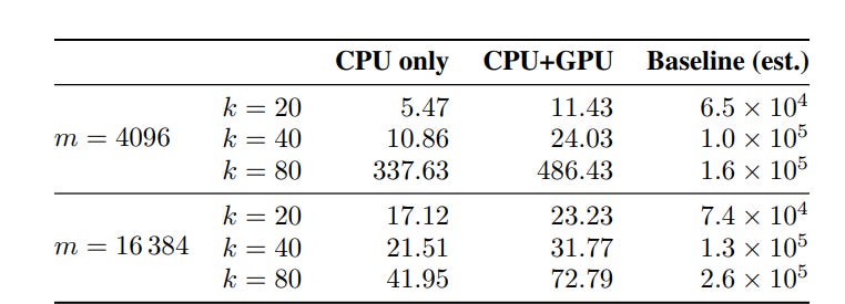
With these cached, the “best atom” search becomes a lookup in DᵀY, and residual updates during Matching Pursuit reduce to cheap additions using DᵀD. In other words, you trade space (large cached matrices) for time (cheap per-iteration work). On modern CPU/GPU nodes with high memory bandwidth, this is a win.
The cost: a massive memory footprint. The gain: a 10,000× speedup. On 2.6M Gemma-2–2B embeddings with m = 4096 atoms and sparsity k = 20, the full algorithm converges in ~8 minutes — versus 30+ days for the baseline.
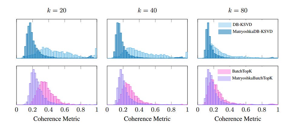
Part B: A New Problem Emerges — Coherence
Scaling exposed a theoretical flaw. The dictionaries DB-K-SVD produced were often highly coherent: many atoms were nearly parallel, representing redundant features. We want the opposite, orthogonal (perpendicular) features, to encode the maximal amount of information.
Formally, coherence μ is the maximum absolute inner product between any two atoms. High μ means the dictionary is crowded with near-duplicates. This is fatal for interpretability:
The sparse encoding step becomes ambiguous — two atoms equally explain the residual.
Sparse codes X become unstable, flipping between redundant atoms.
Distinct monosemantic features blur together.
DB-K-SVD had solved the speed problem, but not the geometry problem.
Part C: The Structural Fix — Matryoshka
The fix was architectural. Borrowing from recent SAE work, the authors imposed Matryoshka structuring —
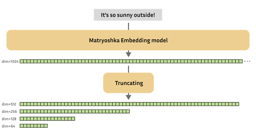
This trains the dictionary in a hierarchy:
Partition the atoms into groups of increasing size.
Train the smallest group (D₁) on the raw data Y. These atoms capture the highest-variance features.
Compute the residual E = Y — D₁X₁.
Train the next group (D₂) on E. By definition, these atoms must capture features unexplained by the first group.
Repeat for deeper groups, each learning to explain the leftovers of the previous stage.
This forces diversity into the dictionary: later groups can’t simply rediscover earlier features. Coherence drops, and interpretability improves.
The trade-off: while autointerpretability and absorption scores rise, some metrics like loss recovery and spurious correlation removal dip slightly. The same pattern appears in Matryoshka SAEs, suggesting this is a structural effect, not an artifact of DB-K-SVD.
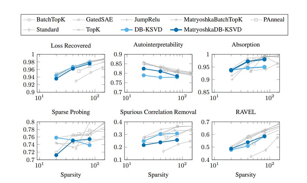
Now we have a speedy algorithm that actually matches the performance of SAEs. In fact, they seem to be nearly identical across the board. What does this tell us? A lot more than you’d think. In research, different methods often compete by outpacing one another: one beats the baseline A, the next beats B , and so on. That’s why we study them to evaluate the tradeoffs.
Here, that didn’t happen. Instead, SAE and DB-KSVD ended up tied. That tie is the signal. It tells us we’re pressing against a ceiling not defined by code or optimizer, but by mathematics.
Section 5: What the Similarity between the DB-KSVD and SAEs tells us
Both methods were tasked with disentangling embeddings from the Gemma-2–2B model and were evaluated on the standardized SAEBench benchmark. As we’ve mentioned, they converged to each other. Two fundamentally different philosophies — one built on stochastic gradient descent and end-to-end training, the other on alternating optimization and explicit updates — both landed in the same neighborhood of performance.
This convergence is strong evidence that the performance limit is not a flaw in our algorithms. The optimizers are working. The limit is a fundamental property of the problem itself, a cage defined by the mathematics of high-dimensional geometry.
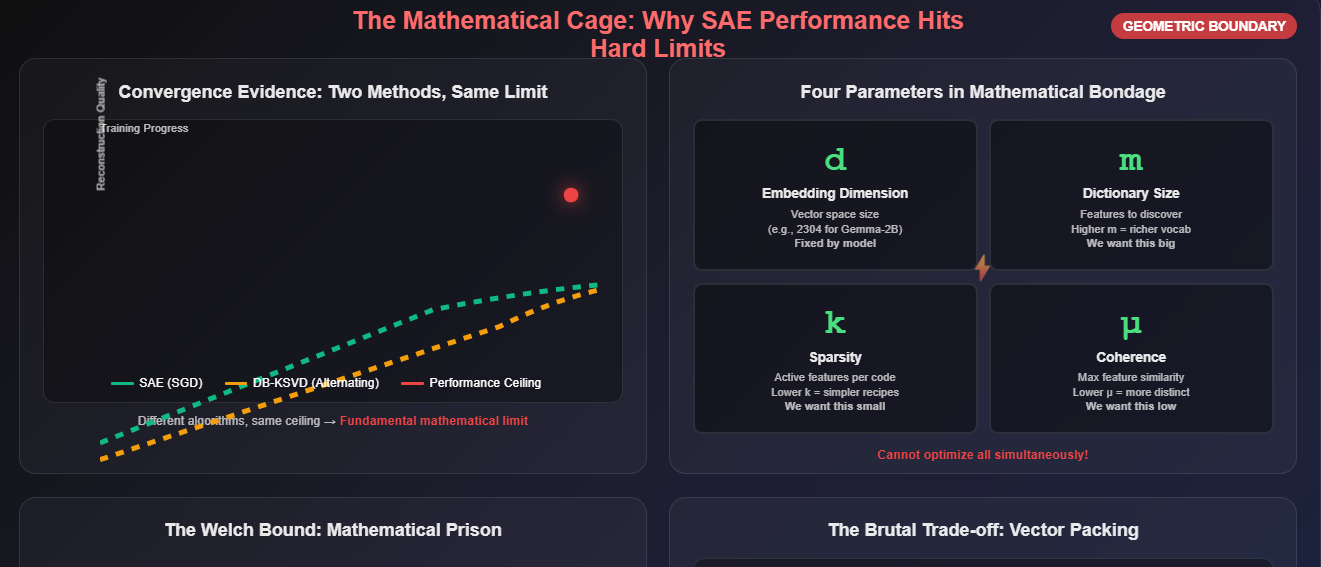
This geometric boundary is governed by a set of inviolable trade-offs between four key parameters:
d (Embedding Dimension): The dimensionality of the vector space. This is the size of the “workspace” provided by the transformer model (e.g., 2304 for Gemma-2–2B).
m (Dictionary Size): The number of monosemantic features we are trying to discover. This is our target vocabulary size.
k (Sparsity): The number of features allowed to be active in any single sparse code.
μ (Coherence): The maximum similarity between any two dictionary features. This measures the geometric distinctness of our learned concepts.
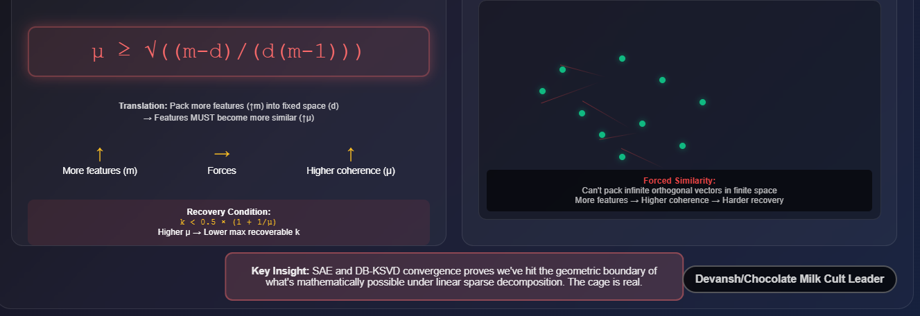
These parameters are not independent. The theory of sparse recovery provides hard mathematical constraints that bind them together. The most critical is the Welch bound, which dictates that as you try to pack more dictionary features (m) into a fixed-dimensional space (d), the minimum possible coherence (μ) must increase. In simpler terms: you cannot pack an infinite number of perfectly distinct (orthogonal) vectors into a finite space. As you add more features, they are forced to become more similar to each other.
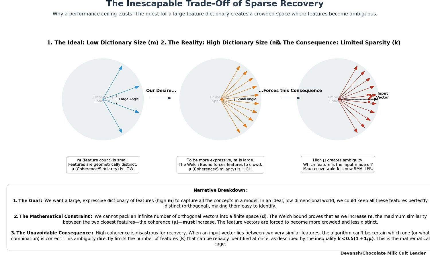
This creates a brutal trade-off. To build a rich, expressive dictionary (high m), we must accept higher coherence (μ). But higher coherence makes the sparse encoding problem harder and less stable. A well-known condition for unique recoverability is k < 0.5 * (1 + 1/μ). As coherence μ increases, the maximum number of features k that can be reliably identified in any given embedding decreases.
Both SAEs and DB-KSVD are implicitly navigating this constrained space. Their convergence suggests they have both found a near-optimal solution within this geometric cage. The performance ceiling we observe is not an algorithmic artifact; it is the boundary of what is mathematically possible under the assumption of linear, sparse decomposition in a high-dimensional Euclidean space.
So where do we go from here?
Section 6. Conclusion: Where do we go from here?
The convergence of DB-KSVD and SAEs at a shared performance ceiling signals the close of one chapter of interpretability research — the search for a scalable linear optimizer — and the beginning of a new one defined by the need to attack the fundamental boundaries of the problem. This is no longer just a software challenge; it is a problem of mathematics and physics. And such, it will require the integration of multiple disciplines.
The path forward is defined by two clear, intertwined trajectories.
1. The Mathematical Frontier: The End of Pure Linearity
The geometric limit of our best linear tools is the strongest evidence to date that the internal representations of transformers are not purely linear. The Y ≈ DX model is a powerful first-order approximation, but we have now likely extracted most of the insight it can offer. To break the current plateau, we must evolve our mathematical toolkit.
The Next Step: Develop non-linear dictionary learning methods. The future lies in tools that can account for more complex geometric structures-
Manifold Learning: Treating features as points on a curved surface rather than vectors in a flat, Euclidean space.
Kernel Methods: Projecting features into a higher-dimensional space where they become linearly separable.
Higher Order Representations of numbers and structures.
Inflection Point to Watch (Scientific): The first credible paper that demonstrates a non-linear method decisively outperforming the SAE/DB-KSVD standard on a benchmark like SAEBench. This will mark the start of a new research paradigm (Est. 2–3 years).
Investing in it early: This is still in the research phase, but if you want to find and fund the next OpenAI/DeepMind within the next 18–24 months, here’s what I’d do —
Allocate capital to a portfolio of 5–7 seed-stage companies (<$5M valuation) founded by PhDs in applied mathematics, theoretical physics, and computational geometry.
Disregard traction. Focus entirely on the mathematical novelty of their approach and its theoretical scaling properties. Avoid any team pitching a “better, faster SAE.”
2. The Physical Frontier: The Memory Wall as a Scientific Barrier
The re-engineering of K-SVD provides a stark lesson in computational physics. Its 10,000x speedup was bought by trading computation for memory. Our ability to run more sophisticated analysis algorithms is now directly constrained by the hardware they run on. No memory, no happiness.
The Hardware Implications: The abstract problem of AI alignment now has a concrete hardware bottleneck. This creates a powerful economic incentive for memory-centric hardware architectures designed not just for training, but for the grueling, memory-intensive work of model introspection. Key technologies include:
Processing-In-Memory (PIM): Moving computation closer to the data to reduce costly transfers.
Advanced High-Bandwidth Memory (HBM): Tighter integration of memory and logic on the same package.
Inflection Point to Watch (Industrial): A major chip designer or cloud provider explicitly markets a new hardware product optimized for “AI analysis” or “model introspection” workloads. I would also monitor for trends like Control as a Service, which is directly reliant on better interpretability. This will signal that the market is finally pricing in the strategic value of trust and reliability (Est. 3–5 years).
Investing in it: Chips and Memory are the best cross-functional investments in the space. We have multiple deep dives on the new stack and the importance of interconnects so look them for details.
Reminder if you want an intro to the Founder Solving for the Memory Wall, shoot me a message — devansh@svam.com w/ details about your fund. I’ll make the introduction. If you want proactive and first-priority matching w/ Founders that match your thesis, get a Founding Member Subscription and email me about it.
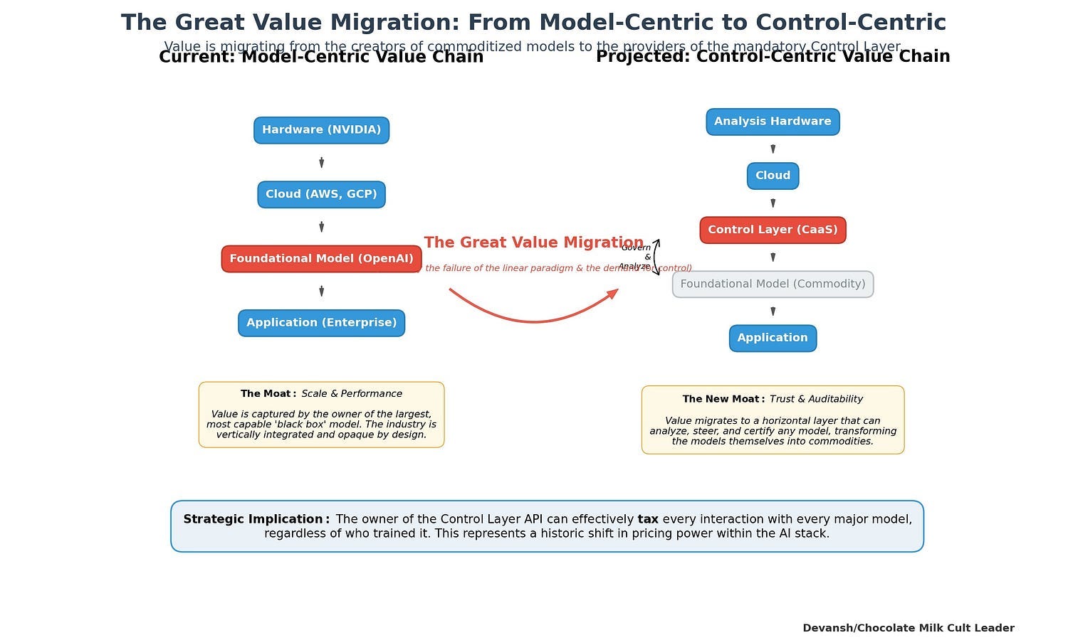
We will touch on all of these in much more detail in our upcoming market deep dive on how to price the AI Interpretability Market, where we’ll price this research (and others), look at the regulatory ecosystem, competing startups, and much more. We’re putting the finishing touches on it and running some of the numbers, but I can promise you that you have a lot to look forward to, such as our analysis on CaaS and how it will change the AI value chain —
There’s a lot to look forward to, and lots to think about. If you learn nothing else from this paper, I hope you will learn the most valuable lesson here — sometimes it might be worth ditching your happy marriage of years, to go back to your ex from 20 years ago, on the off-chance that you can change them to suit your needs.
Thank you for being here, and I hope you have a wonderful day,
Dev <3
If you liked this article and wish to share it, please refer to the following guidelines.
That is it for this piece. I appreciate your time. As always, if you’re interested in working with me or checking out my other work, my links will be at the end of this email/post. And if you found value in this write-up, I would appreciate you sharing it with more people. It is word-of-mouth referrals like yours that help me grow. The best way to share testimonials is to share articles and tag me in your post so I can see/share it.
Reach out to me
Use the links below to check out my other content, learn more about tutoring, reach out to me about projects, or just to say hi.
Small Snippets about Tech, AI and Machine Learning over here
AI Newsletter- https://artificialintelligencemadesimple.substack.com/
My grandma’s favorite Tech Newsletter- https://codinginterviewsmadesimple.substack.com/
My (imaginary) sister’s favorite MLOps Podcast-
Check out my other articles on Medium. :
https://machine-learning-made-simple.medium.com/
My YouTube: https://www.youtube.com/@ChocolateMilkCultLeader/
Reach out to me on LinkedIn. Let’s connect: https://www.linkedin.com/in/devansh-devansh-516004168/
My Instagram: https://www.instagram.com/iseethings404/
My Twitter: https://twitter.com/Machine01776819
This felt like a graduate level course, haha, I learned a lot! Thanks for the breakdown
Thanks for writing this up! This is very interesting.
On a side note, I think to become better memes I've gotta watch more anime.