
How to Train Graph Neural Nets 95.5x Faster[Breakdowns]
How to break the memory wall for large-scale Graph Neural Networks

It takes time to create work that’s clear, independent, and genuinely useful. If you’ve found value in this newsletter, consider becoming a paid subscriber. It helps me dive deeper into research, reach more people, stay free from ads/hidden agendas, and supports my crippling chocolate milk addiction. We run on a “pay what you can” model—so if you believe in the mission, there’s likely a plan that fits (over here).
Every subscription helps me stay independent, avoid clickbait, and focus on depth over noise, and I deeply appreciate everyone who chooses to support our cult.
PS – Supporting this work doesn’t have to come out of your pocket. If you read this as part of your professional development, you can use this email template to request reimbursement for your subscription.
Every month, the Chocolate Milk Cult reaches over a million Builders, Investors, Policy Makers, Leaders, and more. If you’d like to meet other members of our community, please fill out this contact form here (I will never sell your data nor will I make intros w/o your explicit permission)- https://forms.gle/Pi1pGLuS1FmzXoLr6
My crack-cocaine dealer often tells me, “Your network is your net worth”. This advice is also applicable to AI.
Changing the representations of your data is one of the most potent ways to improve the performance of your AI systems. This is the core principle behind Feature Engineering, Prompting, Context Engineering, using different models, and every other technique you know. At their core, all seek to change the way your model perceives (and thus processes) input to nudge for superior responses.
This means that as AutoRegression-based LLMs cap out their potential, we need to look to other methods, other representations, to find the answer. This is where graphs become very promising contenders. Markets, molecules, logistics chains, power grids — our highest-value systems are networks. Whoever learns to model them at the planetary scale wins the next wave of AI.
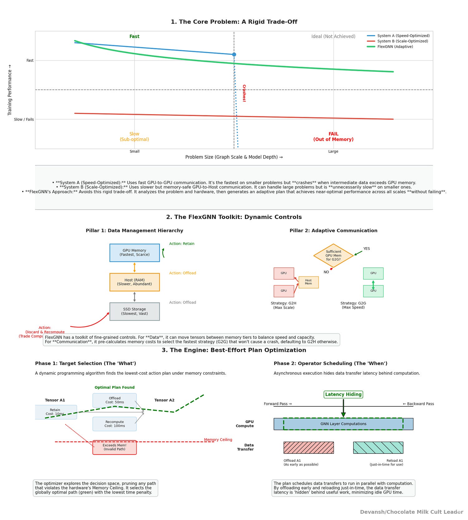
But several challenges stop the large-scale adoption of Graph Neural Nets. Activations balloon to hundreds of gigabytes — larger than the graph itself — while GPUs choke on memory limits and communication bottlenecks. Sampling-based shortcuts exist, but they’re lossy and biased. To unlock the true value of graphs, you need full-graph training — and that has been economically or technically impossible.
“FlexGNN: A High-Performance, Large-Scale Full-Graph GNN System with Best-Effort Training Plan Optimization” is the first credible solution. It reframes training as a system-level optimization problem. Instead of treating GPUs as fixed boxes, it generates a training execution plan that dynamically decides what to keep, what to offload (to RAM or SSD), when to recompute, and which communication path to use.
The result: full-graph training on datasets that previously triggered out-of-memory crashes, and speeds that make prior systems look like prototypes. “Extensive experiments demonstrate that FlexGNN significantly outperforms existing full-graph GNN methods in both training speed and scale. Specifically, it is up to 5.4X faster than HongTu and up to 95.5X faster than NeutronStar.”
This has several major benefits. As it is, it has a lot of potential to unlock a new category of startups and businesses, in two ways —
Picks and shovels: The system layer itself — execution-planning engines that will become as essential as CUDA once was. The winners here supply the infrastructure for the next decade of large-model training, not just in GNNs but in any domain where activations dwarf parameters.
Applied AI: Verticals that live and die by graph structure. Drug discovery and materials science can now simulate molecular interactions at unprecedented resolution. Finance and logistics can finally model risk, fraud, and supply shocks across entire global networks. Social and recommender systems can exploit their rawest data at full fidelity.
The approach (dynamically playing with the resources for custom training schedules) is likely to be one of the unlocks for the memory wall haunting AI across the board, making this paper a must-read for everyone looking to build/invest in the next frontier of AI systems. In many ways, FlexGNN is the Thomas Müller of Vitor Bellforts.
This article will explain this in great detail.
Executive Highlights (TL;DR of the Article)
Graphs are where the highest-value problems in AI live: markets, molecules, logistics, power grids. Whoever masters planet-scale graph modeling takes the next frontier. But full-graph training has been impossible — intermediate activations balloon to hundreds of gigabytes, GPUs choke on memory, and communication between devices becomes a bottleneck
The Breakthrough
FlexGNN reframes training as a system optimization problem:
Memory as a variable: Each intermediate datum can be kept in GPU, offloaded to RAM/SSD, or recomputed — FlexGNN chooses dynamically, balancing cost and speed.
Communication as a variable: Instead of rigid GPU-to-GPU (fast but memory heavy) vs GPU→Host→GPU (slow but scalable), FlexGNN adapts before training begins and overlaps transfers with computation.
Execution plans, not static runs: It generates a pre-optimized training schedule — deciding what to keep, offload, recompute, and when — turning out-of-memory crashes into solvable planning problems.
The Results
Speed: Up to 5.4× faster than HongTu and nearly 100× faster than NeutronStar.
Scale: Trains on graphs with 269M nodes and 4B edges — where other systems fail.
Resilience: Degrades gracefully under memory pressure, shifting to host/SSD offload without collapsing throughput.
Super-linear scaling: Gains more than linear speedup with multiple GPUs by reducing memory pressure
The Implications
FlexGNN proves that software-level planners can unlock orders-of-magnitude efficiency without new silicon. The strategic layer of AI is shifting:
Execution planners (deciding where and how computation runs) are poised to be the next CUDA — the invisible chokepoints that decide feasibility and capture rents.
Verifier systems (deciding what behavior counts as valid) are rising in parallel. Together, they mark the move from monolithic models to modular systems where leverage comes from control layers.
The Economic Shift
Models will commoditize. Control layers calcify. The future of AI won’t be decided by who builds the biggest model, but by who owns the bottlenecks — those filters over memory, bandwidth, and judgment. FlexGNN is a proof-of-concept of this chokepoint economy
I put a lot of work into writing this newsletter. To do so, I rely on you for support. If a few more people choose to become paid subscribers, the Chocolate Milk Cult can continue to provide high-quality and accessible education and opportunities to anyone who needs it. If you think this mission is worth contributing to, please consider a premium subscription. You can do so for less than the cost of a Netflix Subscription (pay what you want here).
I provide various consulting and advisory services. If you‘d like to explore how we can work together, reach out to me through any of my socials over here or reply to this email.
1. The Core Conflict — Why Full GNN Training is Really Hard
1.1 Why Full-Graph Training?
Graph Neural Networks (GNNs) are built to learn from structure, not just features. Each node’s representation emerges from iteratively aggregating its neighbors’ information; the network’s power lies in propagating signals through edges.
There are two ways to train them:
Sampling-based: Break the graph into subgraphs or neighborhoods. This reduces memory pressure and accelerates training but at the cost of bias, variance, and information loss. Neighbor selection becomes an arbitrary bottleneck. Sampling also introduces redundancy — nodes appear across multiple batches, multiplying compute and memory load.
Full-graph (non-sampling): Train on the entire graph at once. No information loss, no sampling bias, no redundant overlaps. Accuracy is consistently higher. This is how GraphCast forecasted global weather and how GNoME discovered millions of new materials.
Full-graph training is the holy grail. It is also computationally unforgiving.
1.2 The Inevitable Crash: The Twin Bottlenecks
Two physical constraints make full-graph training collapse at scale:
Finite GPU Memory. The true villain is not the graph structure itself but the intermediate activations. In a 3-layer GNN on ogbn-papers, the raw graph data is 18.3 GB, vertex data peaks at 71.1 GB, and the intermediate data balloons to 335.9 GB. That’s larger than the combined memory of four 80 GB A100s.

Unfortunately, there’s no way around Intermediate Data; it must persist for reuse in backpropagation. Delete it too early, and you recompute. Keep it all in GPU, and you hit Out-of-Memory before the second epoch.
Finite Communication Bandwidth. Multi-GPU setups don’t eliminate the memory wall; they add a second bottleneck. Each GPU needs the hidden states computed by every other GPU at every layer.
Two strategies dominate:
G2G (direct GPU-to-GPU): Fast, but requires large buffer space in GPU memory.
G2H (GPU→Host→GPU): Slower, but shifts buffers into RAM.
Both strategies are static. Choose wrong and you either crash (OOM on G2G) or crawl (latency-dominated G2H).
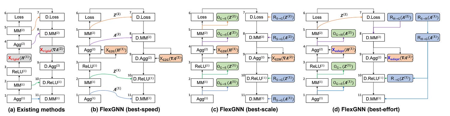
This lays the groundwork for the significance of this work: existing systems make rigid design choices — FlexGNN makes dynamic, cost-aware ones.
How does it do that?
2. Fixing the Problem I — Addressing The Intermediate Data Deluge
As discussed, Full-graph GNN training collapses on activations. Intermediate data points— those temporary results you need later in backprop — balloon to 10–15× the size of the raw graph. So we must find ways to fix this.

2.1 FlexGNN’s Memory Management Toolkit — as an Optimization Space
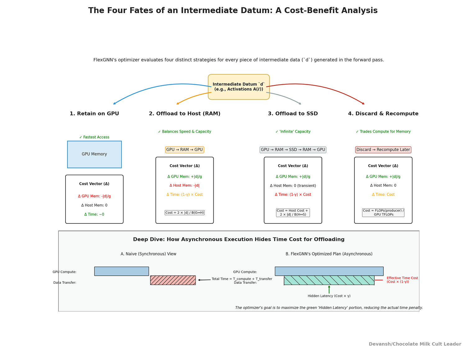
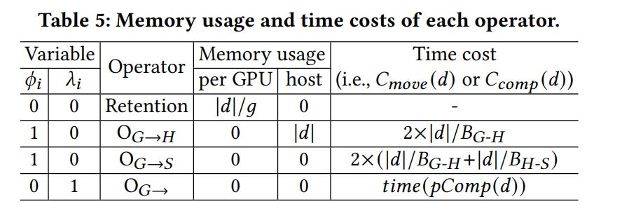
Premise. Every intermediate datum d (e.g., A(ℓ), Z(ℓ) in a GCN) has four legal fates between its forward use and its backward reuse:
Retain (GPU): keep d resident on device; fastest at reuse; consumes |d|/g GPU memory (g = GPUs).
Offload→Host: move d GPU→RAM and later RAM→GPU; time cost = 2×|d| / B(G↔H). This is the middle path, having access to abundant, but still not too slow, memory.
Offload→SSD: move d GPU→RAM→SSD and later SSD→RAM→GPU; cost = 2×(|d|/B(G↔H) + |d|/B(H↔S)). Moving to SSD means you have infinite storage, but your operations will be much slower.
Discard & Recompute: free now; at reuse, recompute the producer op of d; cost ≈ FLOPs(producer) / GPU TFLOPs.
FlexGNN treats “memory residency choices” as first-class nodes in the plan, each with a cost vector (ΔGPU, ΔHost, ΔTime) it can optimize over. Two things make this possible:
Costs are modeled, not guessed. Movement costs are linear in |d| and inversely proportional to measured bandwidths; recompute cost is tied to the exact producing operator’s FLOPs (e.g., MM needs 2×|V|×dim_in×dim_out FLOPs; ReLU needs |V|×dim_out). That table drives the optimizer.
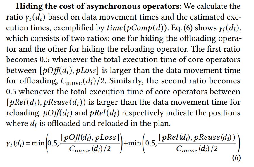
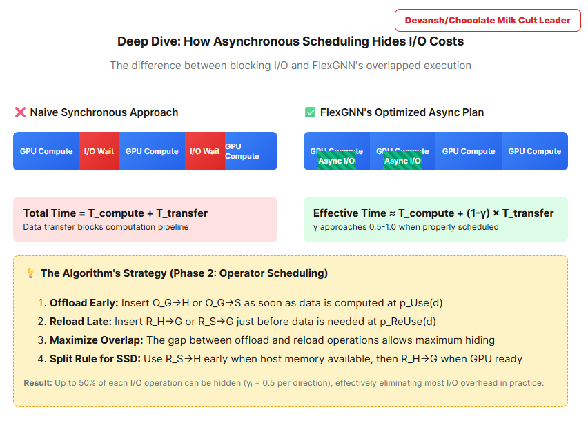
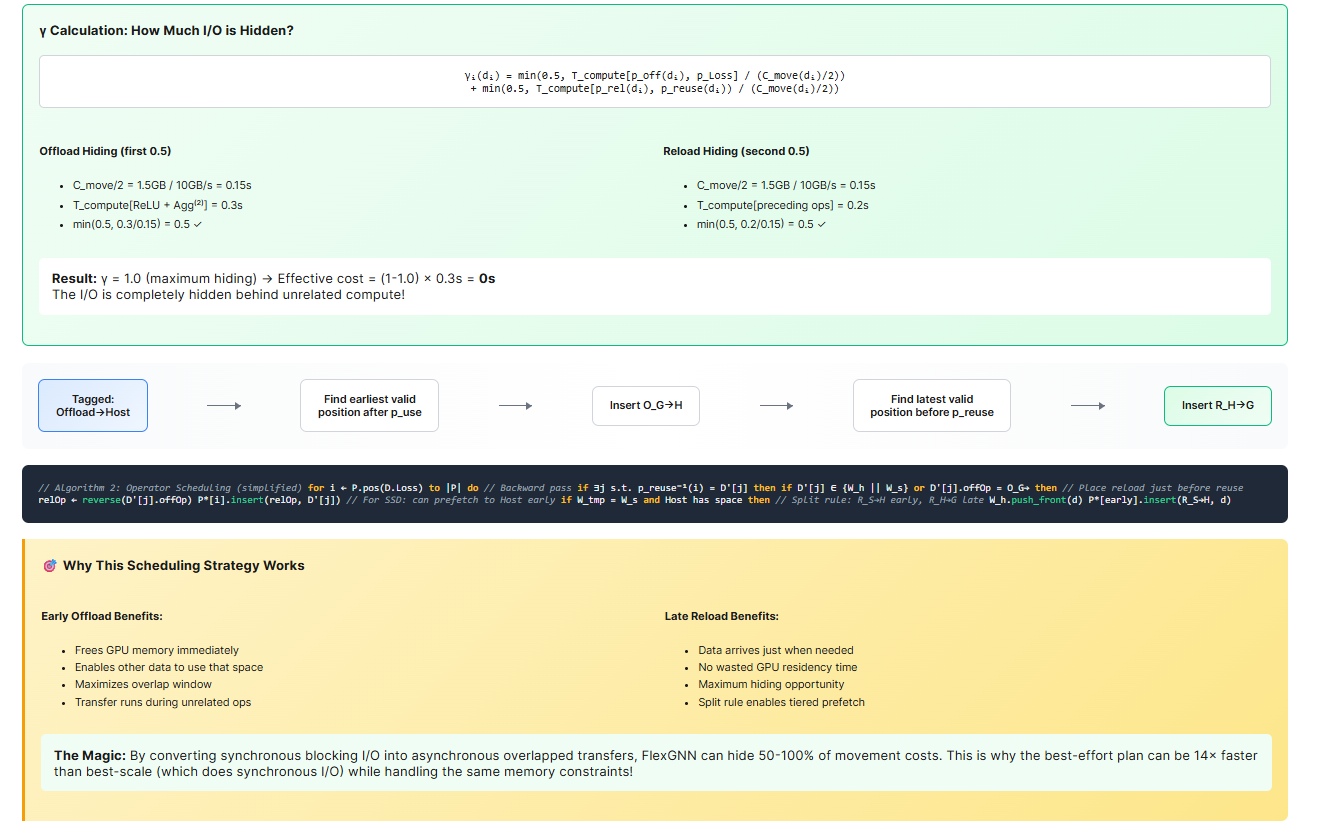
Some movement can be hidden. Because offload/reload run asynchronously beside core ops, a fraction γ(d) of the nominal movement can be buried under compute. The paper formalizes γ(d) as two min(0.5, …) terms — one for offload, one for reload — bounded by the available computation windows before Loss and before reuse. Your effective cost is: effective_move(d) = (1 − γ(d)) × nominal_move(d).
Taken together, each datum d gets a 4-way choice among (Retain | Offload→Host | Offload→SSD | Recompute), with a clear cost comparison at equal units.
This makes the next stage possible.
2.2 Lifetime-Constrained Planning — how decisions are actually made
Now that we have the building blocks of the search in place, we can work on the algorithm for planning.
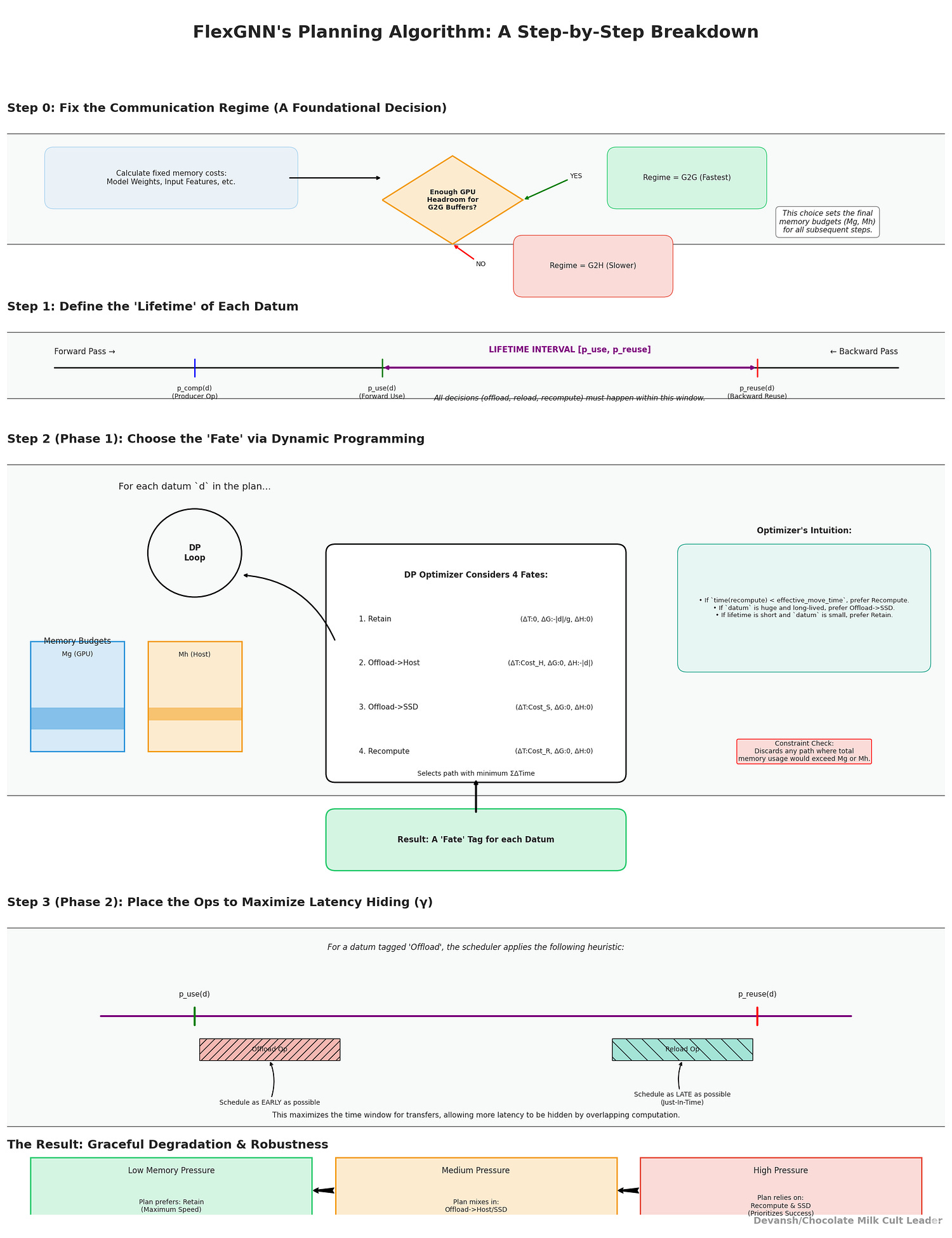
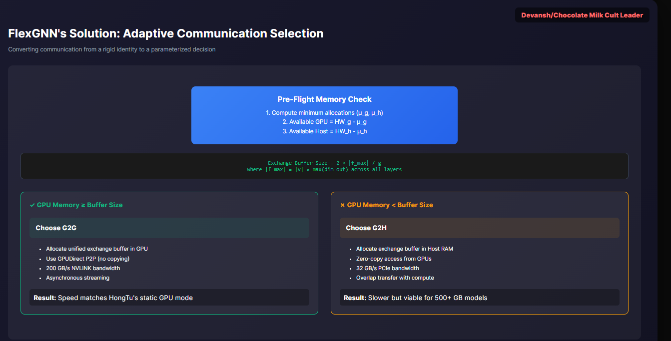
Step 0 — Fix the communication regime. Inter-GPU exchange dominates runtime in full-graph GNNs. FlexGNN first decides G2G vs G2H by checking whether, after reserving model/input/training minima, there is enough GPU headroom to allocate the unified exchange buffer (size 2×|f_max|/g). If yes, choose G2G (faster); else G2H (slower but spares GPU). This determination sets the remaining budgets M_g and M_h for all further choices.
Step 1 — Define lifetimes. For each datum d, the paper defines:
p_comp(d): the op that produces d.
p_use(d): the op that consumes d in forward.
p_reuse(d): the op that needs d’s value in backward (usually the derivative of p_use).
The lifetime interval is [p_use(d), p_reuse(d)]. All offload/reload must lie inside; reload must follow offload; SSD reload may be split (SSD→Host, then later Host→GPU) so you can prefetch into RAM early and acquire GPU memory just-in-time.
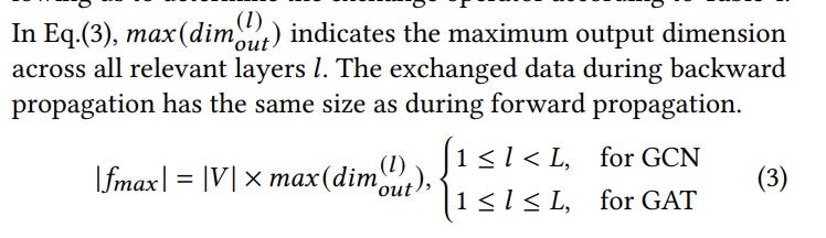
Step 2 — Choose the fate (Phase 1: target selection).
This is a knapsack-over-lifetimes solved via dynamic programming. The optimizer walks the data in plan order and, for each d, considers the four fates with their (ΔGPU, ΔHost, ΔTime) costs:
Retain: time +0, GPU +|d|/g, Host +0.
Offload→Host: time +2×|d|/B(G↔H), GPU +0, Host +|d|.
Offload→SSD: time +2×(|d|/B(G↔H)+|d|/B(H↔S)), GPU +0, Host +0.
Recompute: time +time(p_comp(d)), GPU +0, Host +0.
Crucially, time terms above are later adjusted by γ(d) once scheduling is known; in Phase 1 the DP also adds a small penalty for retaining very long-lived data (adjustCost) so the solver doesn’t greedily squat on GPU with gigantic, long-span activations. It keeps running totals (u_g, u_h) and discards any path that would violate M_g or M_h; among feasible paths, it keeps only the cheapest partial plan. You end Phase 1 with a per-datum tag: retain vs offload-host vs offload-ssd vs recompute.
Intuition on the decision boundary.
For a given d, ignore budgets for a moment and compare effective costs:
Prefer recompute when time(p_comp(d)) < (1 − γ(d)) × movement_cost(d).
(Example: ReLU or cheap MM at small dims.)Prefer offload→Host when movement can be heavily hidden (γ(d) ≈ 1.0 across two halves, capped at 1.0 total), or when recompute is expensive (e.g., Agg with communication).
Prefer offload→SSD only when d is huge and long-lived such that Host would blow M_h; otherwise SSD is a last resort because B(H↔S) is slow.
Prefer retain for short lifetimes (small overlap window → γ(d) small) and/or small d where the residency cost is low and reuse is imminent.
Because all d compete for the same M_g and M_h, Phase 1’s DP doesn’t pick locally greedy actions; it chooses the global combination that keeps the whole plan within budgets at minimum added time. That’s the “formalizing residency” claim made concrete.
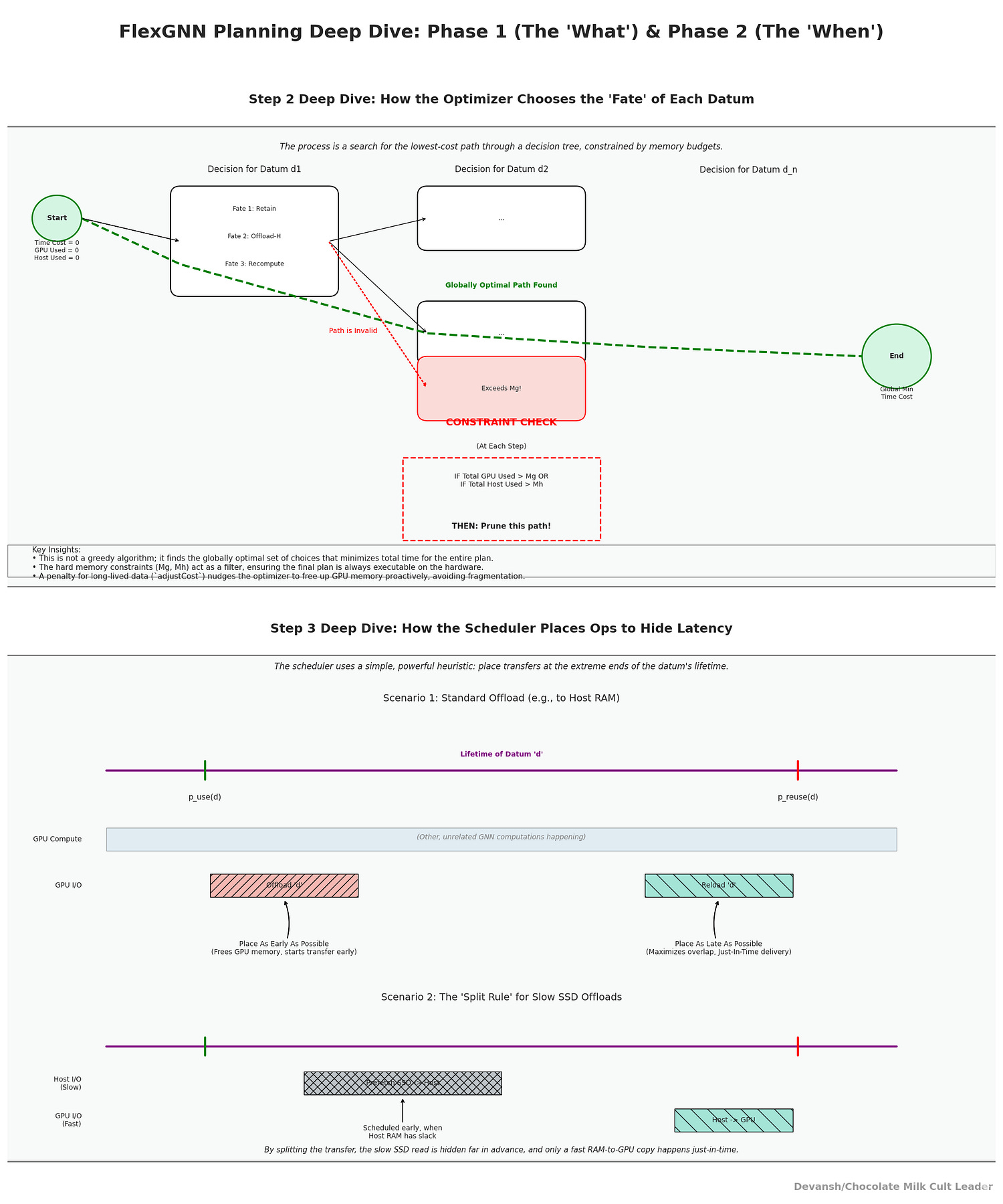
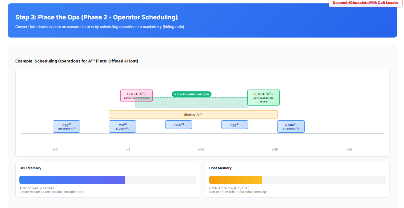
Step 3 — Place the ops (Phase 2: operator scheduling).
Now we convert the tags into an executable plan to maximize γ(d):
Offloads are scheduled as early in the lifetime as memory allows (right after p_use(d)), freeing GPU sooner and enlarging the window in which the offload transfer can run under unrelated compute.
Reloads are scheduled as late as possible (just before p_reuse(d)), giving maximum time to prefetch and overlap the reload. With SSD, FlexGNN can prefetch SSD→Host much earlier (when host has slack) and hold in RAM until GPU space opens; then issue Host→GPU just-in-time. That’s the split rule paying rent.
Retention needs no ops; recompute injects the producer at reuse.
By construction, this increases γ(d) — the hidden fraction of each movement — shrinking effective_move(d) toward zero wherever there is sufficient unrelated compute to mask I/O.
Step 4 — Why this prevents OOM without cratering speed.
If GPU memory tightens, the plan selectively pushes the worst long-lived, expensive-to-retain d into Host or SSD and/or tags cheap producers for recompute.
If Host tightens, SSD absorbs long-tail d while hot paths remain in Host/GPU.
If both are tight, the plan increases recompute on cheap ops and reserves scarce memory for expensive-to-recompute activations.
Exchange regime (G2G vs G2H) is already matched to the budgets, so you don’t die from buffer allocation before the plan even runs.
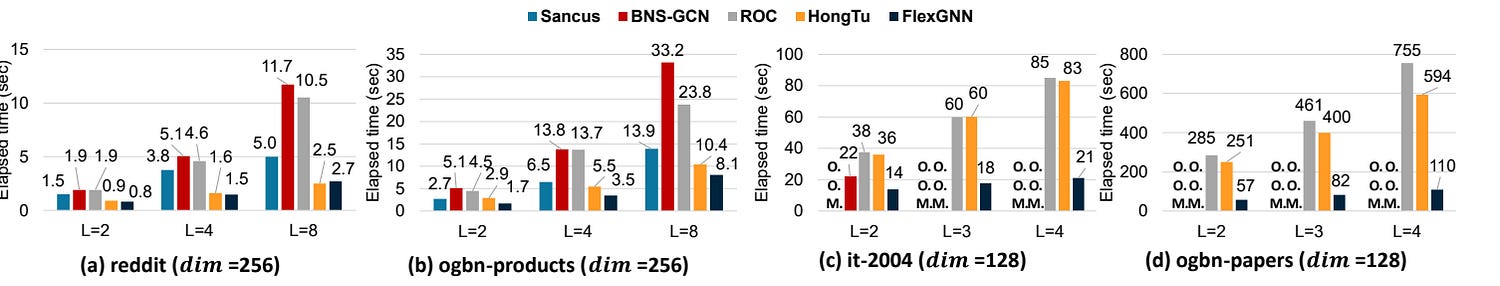
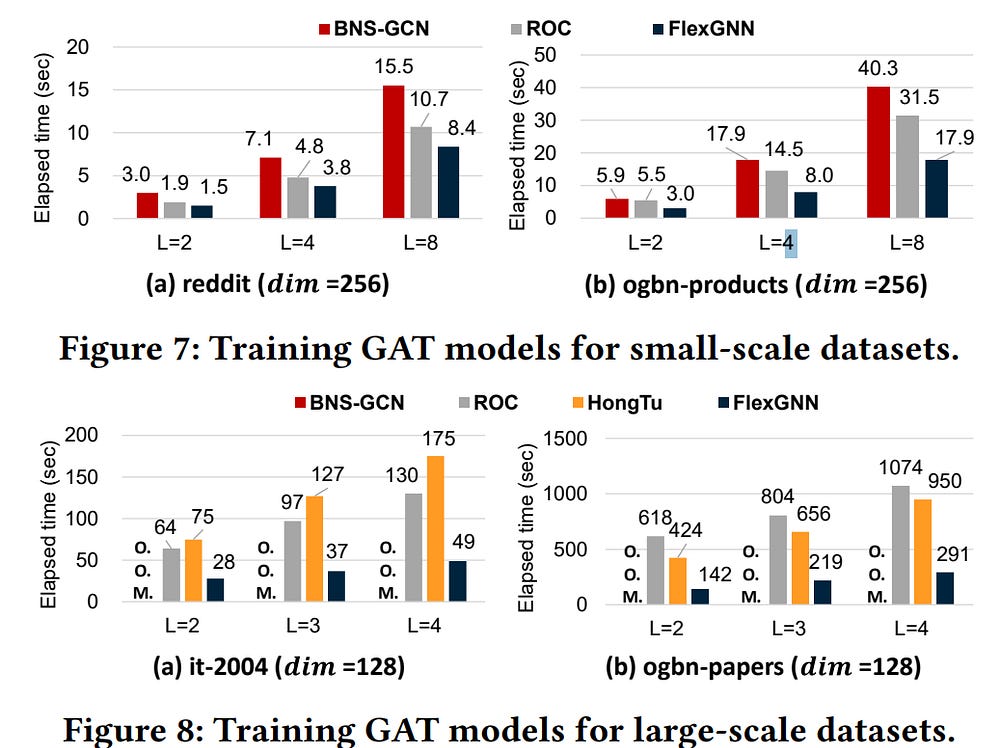
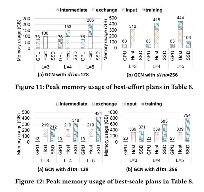
Empirically, that’s why FlexGNN trains models others cannot: e.g., ogbn-papers GCN with dim=256 up to 5 layers (547.8 GB of intermediates) and igb-260m (661.2 GB) succeed by mixing Host/SSD offload and recompute, whereas ROC fails in most of these settings. The best-effort plan matches best-speed when feasible and degrades gracefully when not, beating pure best-scale by up to 14× because movement is overlapped rather than serialized.
One more systems piece that enables this: unified exchange buffers. Instead of per-layer buffers that grow with depth, FlexGNN allocates a double-buffer of size 2×|f_max| (or /g with GPUDirect P2P) and reuses it across layers — keeping the exchange footprint constant while depth grows. That makes the Step-0 G2G decision succeed more often, which in turn lowers movement and frees DP to retain more d in GPU.
The Net effect? “Memory as an optimization variable” isn’t rhetoric here. There is a search space (per-datum fate × legal placement within lifetime) with a budget (M_g, M_h set by the chosen exchange regime) and a modeled objective (sum of movement/recompute minus hidden portions). FlexGNN solves it once, produces a training execution plan, and then runs that plan each epoch. That’s why out-of-memory becomes a planning problem instead of a hard failure mode — and why the resulting runs are fast enough to matter.
3. Fixing the Problem II — How FlexGNN Handles The Inter-GPU Communication Wall
If memory is the first wall, communication is the second. You cannot train a full-graph GNN across multiple GPUs without each device continuously exchanging partial results. Every layer requires that hidden features from one partition be made visible to all others. You need a way to make the GPUs work well together or suffer the same fate as MNM (despite being a GOAT, this showed how much of a system player Messi is, but some of y’all aren’t ready to have that conversation yet).
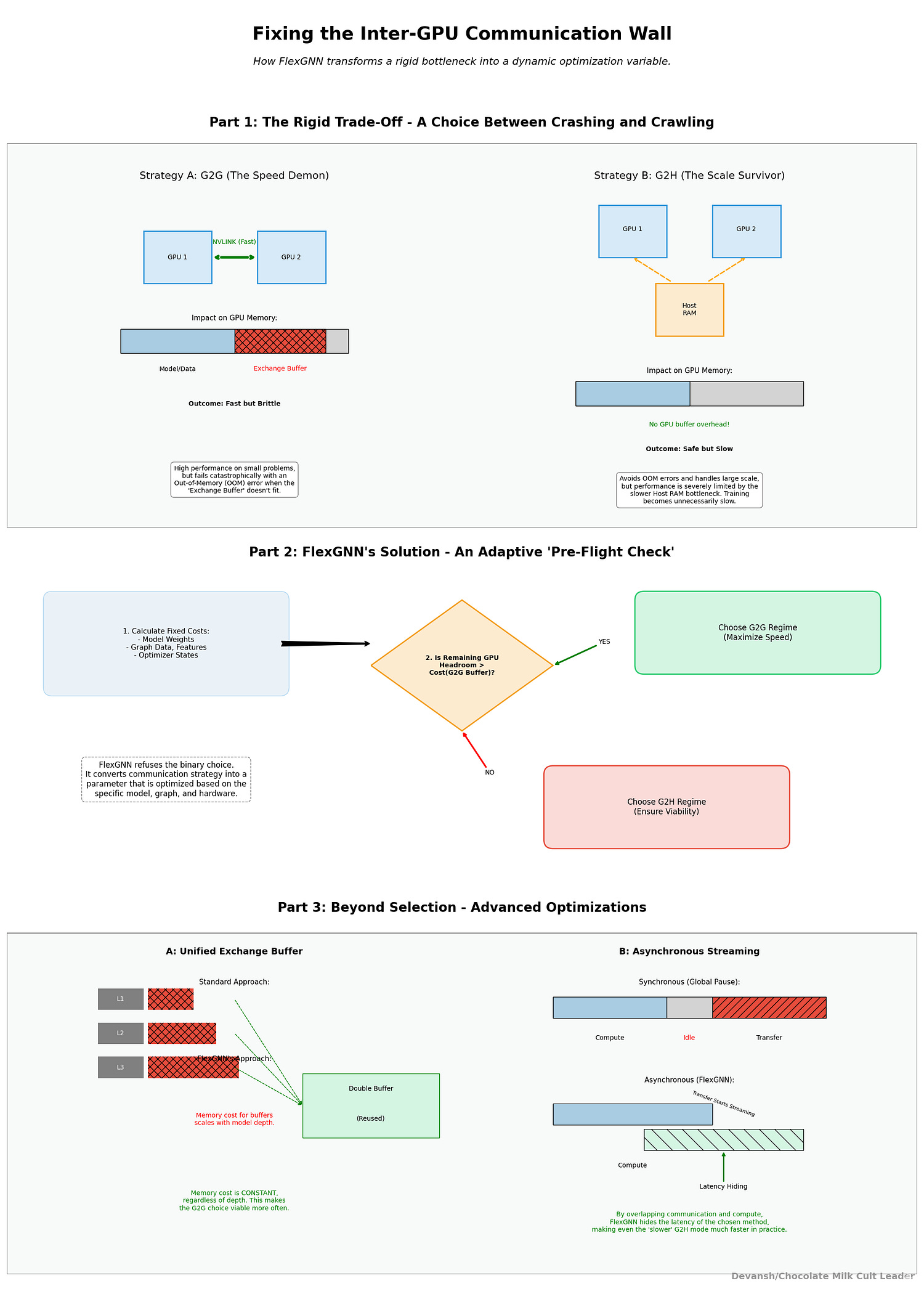
3.1 The Multi-GPU Communication Tradeoff
There are two established strategies:
G2G (GPU-to-GPU direct).
GPUs exchange activations directly over NVLINK or PCIe.
Bandwidth is high, latency is low.
The catch: each GPU must allocate exchange buffers in its local memory. On paper, this is efficient; in practice, those buffers cannibalize the very GPU memory you needed for intermediate activations.
G2H (GPU→Host→GPU).
GPUs spill their activations into host RAM, which acts as a relay.
No GPU buffer overhead, so the model scale can grow larger.
The catch: PCIe is a fraction of NVLINK’s speed, and every transfer is doubled (GPU→Host, Host→GPU). Training slows to a crawl.
The field treated this as binary: either you bet on raw speed (G2G) and accept out-of-memory risks, or you bet on scale (G2H) and accept glacial throughput. Once a system locked into one of these modes, the die was cast (see what I did there; die, dice, hardware; unmatched literary genius here).
3.2 FlexGNN’s Solution — Adaptive Selection
FlexGNN refuses the binary. It evaluates the memory landscape before training begins:
Compute the minimum allocations required: model weights, graph structure, features, labels.
Subtract those from total GPU and host capacities.
Ask: is there enough left to allocate the G2G exchange buffer?
If yes → choose G2G: faster, low-latency training.
If no → choose G2H: slower, but viable when GPU memory is insufficient.
That’s the pre-flight check. It converts communication from a rigid identity to a parameterized decision.
But FlexGNN goes further. Exchange itself is made asynchronous. When a GPU finishes computing its partition, it immediately streams activations into the buffer; aggregation consumes as soon as enough blocks arrive. There is no enforced global pause. Combined with unified exchange buffer management (one double-buffer reused across layers), the communication footprint is flattened. Instead of scaling linearly with depth, buffer cost remains constant.
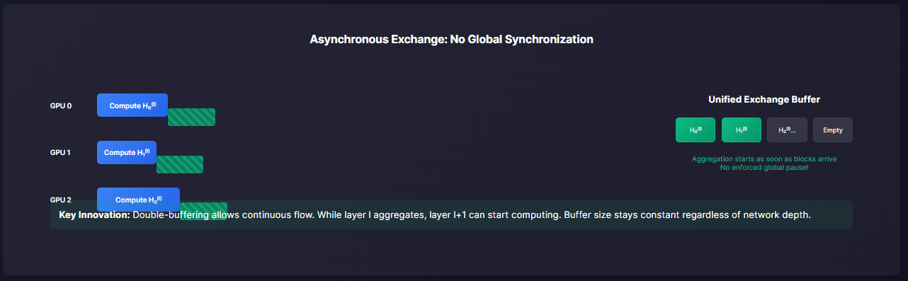
The effect is decisive:
On small graphs, FlexGNN runs with G2G, indistinguishable in speed from HongTu’s static GPU-only mode.
On large graphs where G2G would OOM, FlexGNN downgrades to G2H but overlaps transfer and compute to hide much of the latency.
In practice this balance is why FlexGNN trains ogbn-papers with hundreds of GB of intermediates at 4.9× the speed of HongTu, and why NeutronStar looks prehistoric in comparison.
Taken together, the two pillars — memory management and adaptive communication — form the skeleton of FlexGNN’s design. Memory is no longer a hard ceiling, and communication is no longer a binary lock-in. Both become optimization variables in a global plan.
The next section is where the system’s real genius emerges: how those knobs are actually tuned. FlexGNN doesn’t just provide a toolkit. It generates a training execution plan, a complete, pre-optimized schedule of what to retain, what to offload, when to reload, and how to communicate. That shift — from static execution to dynamic plan generation — is the philosophical break that carries implications far beyond GNNs.
4. What this Means for AI at Large
Before I lay out the investment thesis, let’s play out some of the greatest hits from this system.
4. 1 The Results
Speed: On ogbn-papers, FlexGNN trains a 4-layer GCN (dim=128) 5.4× faster than HongTu and nearly 100× faster than NeutronStar.
Scale: It completes training on igb260m, a 269M-node, 4B-edge graph generating 661 GB of intermediate activations — where ROC and HongTu fail.
Graceful degradation: When memory is abundant, FlexGNN collapses into the best-speed plan. When memory tightens, it degrades to host/SSD offload and recompute — but does so while maintaining usable throughput.
Super-linear speedup: With four GPUs, FlexGNN achieves 4.9× speedup on ogbn-papers. Not from parallel compute alone, but from reducing the memory pressure that hobbled single-GPU runs.
This combination — fast on small graphs, feasible on massive ones — is precisely what sampling-based GNNs and prior full-graph systems failed to deliver.
4.2 The Strategic Implications: The Rise of Control and Verifiers
The gains here come from rethinking execution itself. FlexGNN proves that by treating memory and communication as optimization variables, you can unlock orders of magnitude gains without new silicon.
To me this is a great indication of where the infrastructure market is heading: execution planners that sit above CUDA, orchestrating GPU/CPU/SSD as a tiered hierarchy. This has several advantages —
This will generalize to other forms of Hardware and Interconnects, which will rise to prominence as AI-specific chips and advanced models come into the picture.
Building the above is very CapEx-intensive and risky. Execution planners are not.
Planners will also play a massive role in AI transparency, which will enable the dispersion of AI in high-value, high liability industries. In such cases, trust is generally much more important than intelligence.
Whoever commercializes these systems controls the next bottleneck.
If you read our market report for most important updates in June, your bells are probably ringing. Our report called out the rising importance of reward models and “critics” to steer complex agentic systems. While at the nascent stage right now, these critic models will eventually spawn their own ecosystem to better handle the balance b/w latency, complexity, specific control vectors etc.
This verifier economy will become a crucial part of the AI Stack, especially as AI continues it’s consolidation towards Vertical Plays and Regulation drives an increased focus on Security and Control. The Verifier Economy will change some fundamental assumptions about AI —
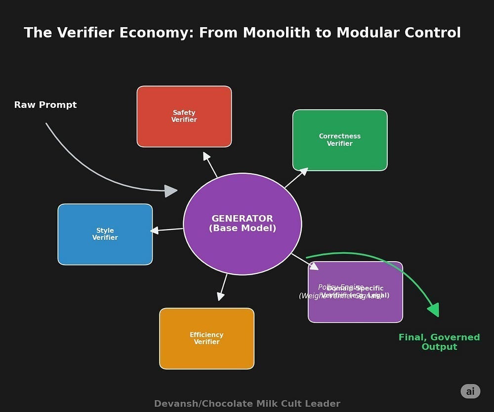
How the Verifier Economy changes the unit of intelligence.
In the LLM era, the unit of progress was the model. In the agent era, it’s the system:
The generator is the actor.
The verifier is the critic.
The task/rubric engine is the environment.
And the simulator is the “world” w/ tools/MCPs being a way to navigate them.
Each of these can be versioned, audited, and improved independently.
Another signal that screams the same trend we’ve been calling for a bit: we’re no longer in monolithic model territory. We’re in modular intelligence. And the leverage has shifted from model size to verifier quality.
This changes the economic layer.
If intelligence is filtered through verifiers, then whoever owns the verifier:
Controls what behavior is considered valid.
Controls what behavior is reinforced.
Controls what behavior becomes dominant across models.
Makes Intelligence composable. Just as APIs allowed developers to assemble complex applications from modular services, verifiers will allow them to assemble complex cognitive agents from modular judgment layers (which is one of the reasons I was interested here to begin with).
Verifiers become programmable incentives. Eventually becoming regulation-mandated standards.
If you wait for the Verifier Economy to show up in sitcoms, you’ll be late to catch the boat. The early players will be able to entrench themselves into the ecosystem, curry favor, and get a huge head start. And while LLMs commoditize aggressively, the Verifier Layer (atleast for more sensitive enterprises) is likely to stay relatively rigid.
I’m pricing the rise of the Verifier Economy first b/c it has earlier timelines for ROI and is in-line with Model Architecture changes that we’re seeing in LLMs. However, dynamic execution is going to be synergistic (or more precisely, verifiers are a part of controllable execution), so it will be best to start monitoring and planning for this accordingly. If models commoditize but verifiers don’t, then the verifier layer captures the durable rents in the AI stack.
5. Conclusion: What FlexGNN can Teach us about the Future of AI
Charles Darwin once taught us that the organisms most capable of change are the ones that will survive. Much of AI has been about optimizing on a base set of assumptions. However, optimized systems are by their very nature, fragile; they sacrifice everything else at the altar of efficiency.
And if history teaches us anything, fashion always swings b/w two poles. Decades of globalization and pro-immigration stances have given way to strong pushes for domestic manufacturing and nationalism. Fatigue around Handcrafted AI gave rise to the Deep Learning (and later LLM) hype, and now we’re seeing a pushback against the non-determinism that made LLMs so appealing. Now, as always, Doestevesky’s Underground Man remains prophetic: “I even think the best definition of man is: a being that goes on two legs and is ungrateful.” No matter what the world gives us, we find flaws and run to the opposite. Every thesis brings an antithesis.
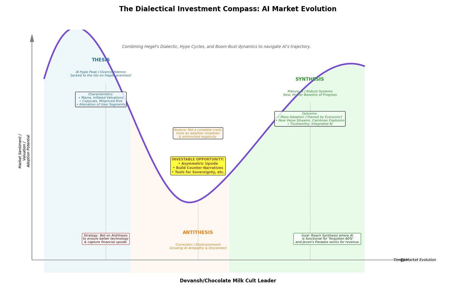
If we are to let the natural course of history take its course, then it’s only natural that the era of AI built on a scaled monoculture will give way to an era where AI works by mixing a diversity of architectures, assumptions, and modalities. Tech like FlexGNNs is then not outlier technologies, but the bell of a new time.
If execution can be planned, then execution can be owned. NVIDIA taught this with CUDA: the API was never just a convenience, it was a control layer. FlexGNN hints at the next iteration: planners that decide what survives in GPU memory, what is shunted to SSD, what is recomputed, and when. Whoever embeds that planner into the stack doesn’t just optimize — they gatekeep feasibility.
And once you see that, the parallel with verifiers is obvious. Hardware planners decide what runs. Behavioral verifiers decide what counts. Both operate as filters between raw capability and usable output. Both become chokepoints. And chokepoints accumulate rents.
The question is not whether execution planners or verifiers work — they do. The question is who monopolizes them, and under what terms. If NVIDIA folds planners into CUDA, the upside accrues to silicon. If regulators mandate standardized verifiers, the upside accrues to whoever controls the rubrics. If neither happens quickly, there is a window — short but real — for independents to define the layer.
FlexGNN is a proof-of-concept. The real story is this: the next frontier of AI won’t be decided by who trains the biggest model. It will be decided by who owns the bottlenecks — those invisible layers where control is exercised over memory, bandwidth, and judgment. Models will blur into a commodity. Control layers will calcify into a monopoly.
That is the chokepoint economy. Fun times ahead.
Thank you for being here, and I hope you have a wonderful day,
Learn from everyone, even (especially?) your crack dealer,
Dev <3
If you liked this article and wish to share it, please refer to the following guidelines.
That is it for this piece. I appreciate your time. As always, if you’re interested in working with me or checking out my other work, my links will be at the end of this email/post. And if you found value in this write-up, I would appreciate you sharing it with more people. It is word-of-mouth referrals like yours that help me grow. The best way to share testimonials is to share articles and tag me in your post so I can see/share it.
I regularly share mini-updates on what I read on the Microblogging sites X(https://twitter.com/Machine01776819), Threads(https://www.threads.net/@iseethings404), and TikTok(https://www.tiktok.com/@devansh_ai_made_simple)- so follow me there if you’re interested in keeping up with my learnings.
Reach out to me
Use the links below to check out my other content, learn more about tutoring, reach out to me about projects, or just to say hi.
Small Snippets about Tech, AI and Machine Learning over here
AI Newsletter- https://artificialintelligencemadesimple.substack.com/
My grandma’s favorite Tech Newsletter- https://codinginterviewsmadesimple.substack.com/
My (imaginary) sister’s favorite MLOps Podcast-
Check out my other articles on Medium. :
https://machine-learning-made-simple.medium.com/
My YouTube: https://www.youtube.com/@ChocolateMilkCultLeader/
Reach out to me on LinkedIn. Let’s connect: https://www.linkedin.com/in/devansh-devansh-516004168/
My Instagram: https://www.instagram.com/iseethings404/
My Twitter: https://twitter.com/Machine01776819