Understanding Microsoft's “Aurora: A Foundation Model of the Atmosphere” [Breakdowns]
How Microsoft AI built a Foundation Model for Climate Forecasting
Hey, it’s Devansh 👋👋
In my series Breakdowns, I go through complicated literature on Machine Learning to extract the most valuable insights. Expect concise, jargon-free, but still useful analysis aimed at helping you understand the intricacies of Cutting-Edge AI Research and the applications of Deep Learning at the highest level.
I put a lot of effort into creating work that is informative, useful, and independent from undue influence. If you’d like to support my writing, please consider becoming a paid subscriber to this newsletter. Doing so helps me put more effort into writing/research, reach more people, and supports my crippling chocolate milk addiction. Help me democratize the most important ideas in AI Research and Engineering to over 100K readers weekly. Many companies have a learning budget that you can expense this newsletter to. You can use the following for an email template to request reimbursement for your subscription.
PS- We follow a “pay what you can” model, which allows you to support within your means, and support my mission of providing high-quality technical education to everyone for less than the price of a cup of coffee. Check out this post for more details and to find a plan that works for you.
Executive Highlights (TL;DR of the article)
Earlier on this year, Microsoft AI quietly dropped the paper, “Aurora: A Foundation Model of the Atmosphere”, where they presented Aurora, a 1.3 Billion Foundation Model for environmental forecasting. The Aurora paper is 52 pages of straight venom, covering various intricacies of building and evaluating foundation models. In this article, our little chocolate milk cult will go deep into the paper to go understand the AI that makes Aurora really special-
Aurora leverages the strengths of the foundation modelling approach to produce operational forecasts for a wide variety of atmospheric prediction problems, including those with limited training data, heterogeneous variables, and extreme events. In under a minute, Aurora produces 5-day global air pollution predictions and 10-day high-resolution weather forecasts that outperform state-of-the-art classical simulation tools and the best specialized deep learning models.
To me, their work is very interesting in its promise of extending to cases with limited training data and predicting extreme events. For example, Aurora was able to predict a vicious sandstorm a day in advance (this is good for sandstorms, which are capricious), which can be used in the future for evacuations and disaster planning- “In a case study, we evaluate Aurora’s predictions for PM10 for 13 June 2023, when Iraq was hit by a particularly bad sandstorm (Figure 27 in Supplementary G.7). Aurora is able to predict the sandstorm a day in advance. This is one in a series of devastating sandstorm events that took place in the late Spring of 2022 leading to more than 5,000 hospitalizations in the Middle East”.
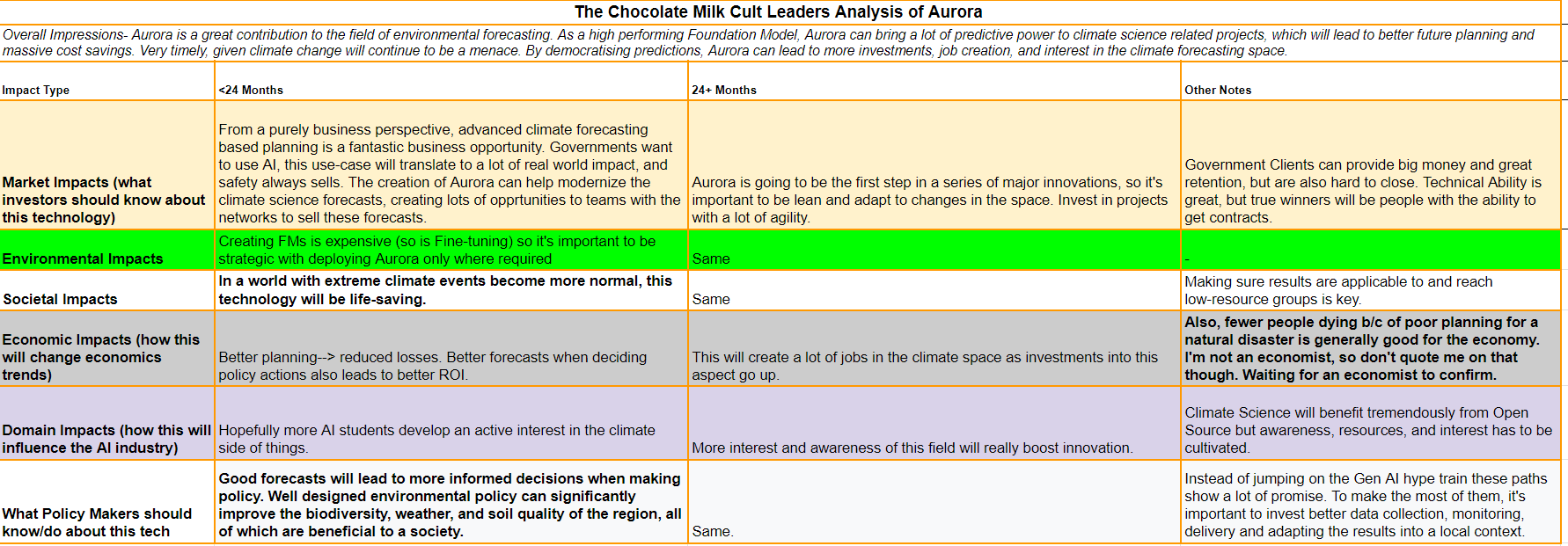
A more detailed exploration of the possible impact of Aurora, including its stonks potential, is given below-
Before we start talking about the technical details, there are 2 things I want to bring up:
Firstly, I will be speculating in a lot of sections (AI researchers, unfortunately, tend not to tell us why they make decisions), so if you have different views- share them. My articles are less “Analysis by a leading authority that should be taken seriously” and more “Speculations by a random dude who learned something cool and wants to start a discussion about it”. I will reach out to the authors of Aurora and ask them to review things (and publish any corrections), but you should also throw in any opinions.
Second- It’s sad that Aurora got almost no attention. To quote the authors- “The ability of foundation models to excel at downstream tasks with scarce data could democratize access to accurate weather and climate information in data-sparse regions, such as the developing world and polar regions. This could have far-reaching impacts on sectors like agriculture, transportation, energy harvesting, and disaster preparedness, enabling communities to better adapt to the challenges posed by climate change” (again, see sandstorm prediction result). This is world-impacting work, but it didn’t even get a proper release from Microsoft. If I search up Aurora on YouTube (which IMO is a pretty good indication of larger community awareness), I get (in this order)-
An AI-generated video from a channel with 60 YouTube Subs.
Amazon posting something unrelated.
A stream by MS with 582 views(where they meander on a bunch of topics, not just Aurora).
A 6 minute vid with a few hundred views
Here are the Screenshots
A Google search isn’t much better, with very little conversation about this development outside of MS websites.
Of all the (non-MS) AI sources I follow- not one has mentioned Aurora in any meaningful capacity. It seems like both Microsoft and the larger AI Community have collectively decided that unreliable chatbots that write our emails and simple code are more important than it. Given how impactful Aurora could be, I think this is a serious misplacement of priorities, and I hope more people remember that there are very important problems outside of LLMs and GenAI.
Anyhoo, if you’re convinced about the utility of this technology, here is an overview on how the MS researchers cooked up Aurora.

Following are the different components + their rationale. This will get to be a lot (the researchers solved a lot of different things) so grab some milk, and we’ll dance through these one at a time.
1. 3D Perceiver Encoder (Section B.1):
Challenge: Weather data is heterogeneous (different variables, resolutions, pressure levels). Traditional models struggle with this.
Solution: Aurora uses a 3D Perceiver encoder to map diverse datasets into a standardized 3D tensor.

Why Perceiver? Perceivers are good at handling varying input sizes and modalities, making them ideal for heterogeneous weather data.
Level Embeddings: Each input patch is embedded into a vector and tagged with a level encoding (pressure level or surface). This helps the model understand the vertical structure of the atmosphere.
Level Aggregation: Perceiver modules reduce the number of pressure levels to a fixed set of latent levels, enabling efficient processing.
2. Multi-Scale 3D Swin Transformer U-Net Backbone (Section B.2)

Challenge: Simulating atmospheric dynamics requires capturing interactions across different spatial scales.
Solution: Aurora uses a 3D Swin Transformer U-Net backbone.
Why Swin Transformer? Swin Transformers excel at capturing long-range dependencies and scaling to large datasets, which is crucial for weather modeling.

Why U-Net? The U-Net architecture allows for multi-scale processing by downsampling (reducing dimensions) and upsampling (increasing the dimensions) the data, enabling the model to learn features at different resolutions: “This structure enables the backbone to simulate the underlying physics at multiple scales.”
Local Self-Attention: Swin Transformers use local self-attention within windows, reducing computational complexity while still capturing local interactions.
Window Shifting: Shifting the windows every other layer allows for information exchange between neighboring regions, mimicking the flow of information in the atmosphere. I don’t know enough about Climate Models to know if this is standard practice, but imo this is super duper clever.
3. 3D Perceiver Decoder (Section B.3):

Challenge: Decoding the standardized output back to the original variables and resolutions.
Solution: Aurora uses a 3D Perceiver decoder, mirroring the encoder’s structure.
Why Perceiver?- Same as above.
Level De-aggregation: Perceiver layers expand the latent atmospheric levels back to the original pressure levels.
Patch Reconstruction: Linear layers decode the latent representations into patches, which are then combined to form the final output. “Analogously to the patch embedding layer in the encoder, the linear layer constructing the output patches is constructed dynamically by selecting the weights associated with each variable. This overall architecture allows the decoder to output predictions at arbitrary pressure levels, for an arbitrary set of variables.”
4. Data Normalization (Section B.5):
Challenge: Weather variables have different scales and distributions.
Solution: Aurora normalizes each variable separately using a spatially constant scale and center, estimated from the ERA5 training data.
Why ERA5? ERA5 is a high-quality reanalysis dataset, providing a reliable basis for normalization.
Benefits: Normalization improves model stability and convergence during training.
5. Extensions for 0.1° Weather Forecasting (Section B.6):
Note- AFAIK, The term “0.1° weather forecasting” refers to high-resolution weather forecasting with a spatial resolution of 0.1 degrees latitude and longitude. Correct me if I’m misunderstanding this, I couldn’t find an explanation in the paper.
Challenge: High-resolution data requires significant memory.
Solutions:
Patch Size Increase: Increasing the patch size reduces the number of tokens, lowering memory requirements.
Remove Backbone Layers: Removing some layers from the backbone further reduces memory usage without significantly impacting performance
6. Extensions for Air Pollution Forecasting (Section B.7):
Challenge: Air pollution variables are sparse and have a large dynamic range.
Solutions:
12-Hour Model: A separate model pretrained with a 12-hour time step is used to capture diurnal cycles in pollutants.
Differencing: The model predicts the difference with respect to a previous state, improving accuracy for variables with strong diurnal cycles.
Specialized Normalization: A custom normalization scheme is used for air pollution variables to handle their sparsity and dynamic range.
Transformation of Concentration Variables: A combination of the original variable and its logarithm is used to capture both high and low-magnitude values.
Additional Static Variables: Static variables related to time of day, day of week, and emissions are included to provide additional context.
Variable-Specific Clipping: “SO2 at 850 hPa and above tends to be particularly spikey. To help stabilise roll-outs, during and after LoRA roll-out fine-tuning, we clip the predictions only for SO2 at 850 hPa and above at 1. This clipping happens before unnormalisation.”- This helps prevent extreme values from destabilizing the model during long-term forecasting.
Patch Size Decrease: “The lower resolution of CAMS analysis data (0.4◦ instead of 0.25◦) allows us to use a smaller patch size of 3 instead of patch size 4. To ensure maximum transfer, we initialise the size 3 patches”- smaller patch sizes should increase performance.
Pressure-Level-Specific Patch Embeddings: To account for the different behaviors of air pollution variables at various altitudes (different levels of human influence), the encoder and decoder patch embeddings depend on the pressure level. This allows the model to learn more specialized representations of different parts of the atmosphere.
Additional 3D Perceiver Decoder: A separate 3D Perceiver decoder is used specifically for air pollution variables. This helps the model learn distinct features for these variables, improving prediction accuracy.
32-bit Floating Point Computation: To better handle low-magnitude values, computations before and after the backbone are performed in 32-bit floating point precision. This increases numerical accuracy and stability, especially for sparse air pollution variables.
I will skip section C (datasets) because I have nothing meaningful to add there. Look at it when building around/evaluating Aurora.
7. Training Objective (Section D.1):
Objective: Mean Absolute Error (MAE) is used as the training objective.
Why MAE? MAE is robust to outliers. We’ve discussed this idea at length in our discussion on jailbreaking multimodal models, but to summarize- squaring your error (as you would with MSE) tends to ignore small errors and disproportionately punish large ones-
In an outlier-heavy field like Climate, this can make learning the behavior extremely noisy. If you throw lots of huge outliers at it, MAE won’t lose it’s shit the same way MSE would, making it much better here.

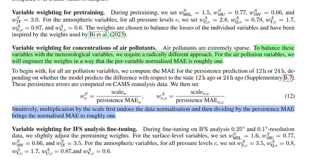
Variable Weighting: Different weights are assigned to different variables to balance their contributions to the loss. What they did with the pollutants vars was particularly interesting.
Rationale: This ensures that all variables are learned effectively, even those with small magnitudes or sparse distributions.
8. Training Methods (Sections D.2-D.4):
Pretraining: The model is first pretrained on a massive dataset of weather and climate data.
Benefits: Pretraining allows the model to learn general representations of atmospheric dynamics, which can then be adapted to specific tasks.
Short Lead-Time Fine-tuning: The pretrained model is fine-tuned on specific tasks using a small number of rollout steps.
Purpose: This adapts the model to the specific task and improves short-term forecasting accuracy.
Roll-out Fine-tuning: Low Rank Adaptation (LoRA) is used to fine-tune the model for long-term multi-step dynamics. There is some other nuance, that we’ll touch up on when we get to the relevant section.

Why LoRA? LoRA is a memory-efficient method for fine-tuning large models, enabling long-term forecasting without exceeding memory limits.
And that is a summary of the AI behind Aurora. If you understand all the components, let’s now discuss the algorithmic ideas in more detail to get a better picture of what makes the Foundation Model work so well.
I put a lot of work into writing this newsletter. To do so, I rely on you for support. If a few more people choose to become paid subscribers, the Chocolate Milk Cult can continue to provide high-quality and accessible education and opportunities to anyone who needs it. If you think this mission is worth contributing to, please consider a premium subscription. You can do so for less than the cost of a Netflix Subscription.
I provide various consulting and advisory services. If you‘d like to explore how we can work together, reach out to me through any of my socials over here or reply to this email.
Taming Heterogeneous Weather Data with the 3D Perceiver Encoder
There are 3 major differences between climate data and text, which makes creating Foundation Models for Climate harder-
Unlike text, which is relatively uniform, weather datasets come with a mix of variables (temperature, wind speed, humidity, etc.), different resolutions (spatial grid sizes), and varying pressure levels (representing different altitudes in the atmosphere). Traditional deep learning models, often designed for homogeneous data, struggle to handle this variability.
Weather data is a lot less self-contained (it’s more likely to be influenced by components that are not being measured).
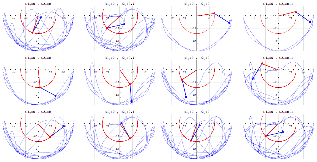
Weather is chaotic, which makes it sensitive to the smallest differences. This can be a death sentence for training large scale models (the effort required to prune and manage large scales of data to make sure it’s good is very high)-
These 3 differences combine to form a very special kind of menace when it comes to creating joint embeddings for the varying types of weather data. So, how do we beat this triple threat into submission? The key is in their use of 3d Perceivers. Perceivers, a type of Transformer, are particularly adept at processing inputs with varying sizes and modalities. They achieve this by using cross-attention, where a set of learnable queries attends to the input data, regardless of its structure.

This allows Aurora to process weather data from different sources and resolutions without requiring extensive preprocessing or architectural modifications.
Biological systems perceive the world by simultaneously processing high-dimensional inputs from modalities as diverse as vision, audition, touch, proprioception, etc. The perception models used in deep learning on the other hand are designed for individual modalities, often relying on domain-specific assumptions such as the local grid structures exploited by virtually all existing vision models. These priors introduce helpful inductive biases, but also lock models to individual modalities. In this paper we introduce the Perceiver — a model that builds upon Transformers and hence makes few architectural assumptions about the relationship between its inputs, but that also scales to hundreds of thousands of inputs, like ConvNets. The model leverages an asymmetric attention mechanism to iteratively distill inputs into a tight latent bottleneck, allowing it to scale to handle very large inputs. We show that this architecture is competitive with or outperforms strong, specialized models on classification tasks across various modalities: images, point clouds, audio, video, and video+audio. The Perceiver obtains performance comparable to ResNet-50 and ViT on ImageNet without 2D convolutions by directly attending to 50,000 pixels. It is also competitive in all modalities in AudioSet.
-Perceiver: General Perception with Iterative Attention. I haven’t rated this paper super highly so far, but this seems to be key for sucess. My apologies to the Perceiver transformer crew, I was not familiar with your game.
We add to this by incorporating level embeddings. Each input patch, representing a small region of the atmosphere, is embedded into a vector and tagged with a level encoding. This encoding indicates either the pressure level (for atmospheric variables) or the surface level. By explicitly representing the vertical structure of the atmosphere, the model can better understand the relationships between variables at different altitudes.
Finally, the encoder uses another Perceiver module to aggregate the information from the physical pressure levels into a fixed set of latent levels. This aggregation serves two purposes: it enables efficient processing by reducing computational complexity, and it creates a standardized representation that can be used across different datasets with varying vertical resolutions.
We now have our patches. The next step is to take these patches and run them through the simulation. That is where our backbone comes in to play.
Simulating Atmospheric Dynamics with a Multi-Scale 3D Swin Transformer U-Net Backbone
If the 3D tensor that the backbone receives as input can be viewed as a latent 3D mesh on which the simulation is performed, then the backbone can be viewed as a (neural) simulator. Transformers, due to their proven scaling properties (Kaplan et al., 2020) and connections with numerical integration (Brandstetter et al., 2022), are a natural architectural choice for this simulation engine. To this end, we opt for a 3D Swin Transformer U-Net (Liu et al., 2021, 2022) architecture
Our embeddings provide us with very promising raw material. But we need something very special to turn an Overeem into Ubereem. And that is what our backbone does. For accurate long-term forecasts, we need a model architecture that simultaneously processes and understands atmospheric phenomena at various scales while maintaining computational efficiency. Let’s talk about the 1–2 combo that forms the basis of Aurora’s backbone: the Swin Transformer and the U-Net structure. This combination allows the model to efficiently capture both long-range dependencies and local interactions across multiple scales.
Let’s break ’em down, one at a time. Please note that Aurora mashes them (it’s a UNet shaped Swin Transformer). I’m distinguishing them to explain the significance of each.
Swin Transformer: Capturing Long-Range Dependencies
The key innovation of Swin Transformers is their use of shifted windows for self-attention computation. Unlike standard Vision Transformers that compute self-attention globally (which leads to quadratic computational complexity), Swin Transformers compute self-attention only within local windows. This approach has two major advantages:
Linear Computational Complexity: By restricting attention to local windows, the computational complexity scales linearly with the input size, allowing the model to handle much larger inputs.
Hierarchical Feature Representation: The architecture builds hierarchical feature maps by merging patches in deeper layers, similar to how convolutional neural networks create increasingly abstract representations.
One thing that makes Swin Transformers really ideal for this is it’s shifted window, which allows for information sharing between patches, which models the constantly dynamic interaction b/w an atmospheric patch and it’s neighbors.

These properties make Swin Transformers ideal for weather modeling, where we need to process large amounts of data and capture both local and global patterns.
Before we move on, reading this gave me a thought. I’ve been toying with the idea of Fractal Based Compression (both for language and images)-
Given how good they are with modeling chaotic systems, I wonder if there is some use in combining Fractal Based Compression with these embeddings. Essentially use Fractals to encode the less important parts of the input, leaving you with most resources on the more salient features.
I have mixed feelings here-
Weather being chaotic, might not respond well to downsampling away some information (even if we only touch the less important bits).
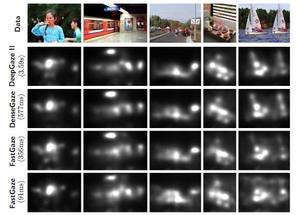
The “Faster gaze prediction with dense networks and Fisher pruning” paper showed us that heavily pruned networks still create very similar saliancy maps. We might be able to get away with something here.
I have no strong leanings either way, so I’m curious to hear what y’all have to say about this.
For now, we move on. The Swin Transformer sets us up. Every strong opener needs a strong close and our backbone does it the following-
U-Net Structure: Enabling Multi-Scale Processing
The U-Net architecture, originally developed for biomedical image segmentation, has proven to be a powerful tool for tasks requiring multi-scale understanding. In Aurora, the U-Net structure is adapted to work with the Swin Transformer layers.
The U-Net consists of an encoder path that progressively downsamples the input, followed by a decoder path that upsamples the features back to the original resolution.

This structure allows the model to:
Capture features at multiple scales: The encoder path creates a hierarchy of features at different resolutions.
Combine low-level and high-level information: Skip connections between the encoder and decoder allow the model to integrate fine-grained spatial information with more abstract, contextual information.
In the context of weather modeling, this multi-scale processing is crucial. It enables Aurora to simultaneously understand local weather patterns and larger-scale atmospheric phenomena, mirroring the multi-scale nature of real atmospheric dynamics.
This combination is the Son-Kane duo of Machine Learning (except this wins trophies).
We’ll skip the rest of section B b/c I really don’t have much to add to it.
Let’s start our discussion on the actual training of Aurora. And wow, we’ve got things to talk about.
Training Objective for Aurora
If you’re reading this, I think I can trust in your intelligence to understand that MAE Big Brothers MSE inn high outlier scenarios, so we want to build around that as our error metric.
The problem is that a naked MAE isn’t good enough for us. Different weather variables have different importance and exhibit different levels of variability. For example, accurately predicting temperature is generally more critical than predicting specific humidity, and wind speed tends to be more variable than geopotential height. To account for these differences, Aurora uses variable weighting, where different weights are assigned to different variables in the loss function. This ensures the model focuses on learning the most important and challenging variables, leading to more accurate and balanced forecasts.
Now, the authors could have used a hard-coded scheme to make this breakdown much easier, but instead, we are stuck with Lovecraft’s long-lost Outer God-
This looks bad, but once you understand the basic components, this looks much easier. Overall, this is a weighting scheme to balance the contributions of different variables to the loss function. Let’s break down the formula (one question: why don’t people use a and b instead of Greek letters, typing the former is so much easier):
L(X̂^t, X^t) = (γ / (V_S + V_A)) [ α (…) + β (…) ]
V_S: Number of surface-level variables
V_A: Number of atmospheric variables
γ: Dataset weight (varies by dataset quality)
α: Weight for surface variables (set to 1/4)
β: Weight for atmospheric variables (set to 1)
The loss is decomposed into two main parts:
Surface-level Variables: α (Σ[k=1 to V_S] w^S_k (1/(H×W)) Σ[i=1 to H] Σ[j=1 to W] |Ŝ^t_k,i,j — S^t_k,i,j|)
w^S_k: Weight for each surface-level variable
H, W: Height and width of the spatial grid
Ŝ^t_k,i,j, S^t_k,i,j: Predicted and true values for surface variable k at position (i,j)
Atmospheric Variables: β (Σ[k=1 to V_A] (1/(C×H×W)) Σ[c=1 to C] w^A_k,c Σ[i=1 to H] Σ[j=1 to W] |Â^t_k,c,i,j — A^t_k,c,i,j|)
w^A_k,c: Weight for each atmospheric variable at each pressure level
C: Number of pressure levels
Â^t_k,c,i,j, A^t_k,c,i,j: Predicted and true values for atmospheric variable k at level c and position (i,j)
Along with this, we have this-
Here is my thinking on why the whole thing is structured in the way it is-
Balancing Surface and Atmospheric Variables: By using separate weights (α and β) for surface and atmospheric variables, the model can balance its learning between these two domains. The choice of α = 1/4 and β = 1 suggests a greater emphasis on atmospheric variables, possibly due to their higher dimensionality and complexity.
Variable-Specific Weighting: The weights w^S_k and w^A_k,c allow fine-grained control over the importance of each variable. This is particularly useful for handling variables with different scales or importance to the forecasting task. This is probably done so that Aurora can be plugged into different fine-tuned cases and adapted to them easily.
Dataset Quality Consideration: The γ factor allows the model to prioritize learning from higher-quality datasets (like ERA5 and GFS-T0) during training. This is a good way to incorporate prior knowledge about data reliability into the learning process.
Spatial Averaging: The summations over H and W, divided by the grid size, effectively compute spatial averages. This ensures that regions with different resolutions are treated fairly in the loss computation.
The model can effectively learn from diverse weather variables across different spatial scales and data sources by using MAE as the base metric and incorporating a sophisticated weighting scheme. This objective function is a key factor in Aurora’s ability to handle the heterogeneous and complex nature of weather data, contributing to its impressive performance across various forecasting tasks.

This is then leveraged into the training. Tbh, I didn’t think there was much remarkable about the Pretraining and Short-lead tuning, so I will not talk about them. But the roll-out fine-tuning was pretty interesting, so let’s end with a discussion of that.
Mastering Long-term Dynamics with Roll-out Fine-tuning
To ensure long-term multi-step dynamics, AI models typically fine-tune the model specifically for rollouts. Backpropagating through the auto-regressive rollouts for a large number of steps is unfeasible for a 1.3B parameter model such as Aurora. This is particularly true at 0.1◦ resolution, where even a single step rollout is close to the memory limit of an A100 GPU with 80GB of memory.
Imagine you’re trying to predict where a billiard ball will go after you hit it. Predicting the next few bounces might be relatively easy. But what about predicting the ball’s path over many bounces, as it ricochets off the cushions and interacts with other balls? That’s a much harder problem!
Weather forecasting is similar. Predicting the weather a few hours ahead is one thing, but making accurate predictions for days or even weeks into the future is a much more complex challenge. This is where “rollout fine-tuning” comes in. It’s a specialized training technique that helps Aurora master the art of long-term weather prediction.
Rollout fine-tuning addresses this challenge by training Aurora on sequences of multiple predictions, simulating the chain reaction of weather events over time. Think of it like this:
Start with a Snapshot: Aurora is given a snapshot of the current weather conditions.
Predict the Next Step: Aurora makes a prediction for the weather a few hours ahead.
Feed the Prediction Back: Aurora then uses its own prediction as input to predict the weather even further ahead.
Repeat: This process is repeated multiple times, creating a chain of predictions that extends into the future.
By training on these rollout sequences, Aurora learns to account for the long-term consequences of its predictions, improving its ability to forecast weather patterns over extended periods.
Here are the Key Innovations that make this work:
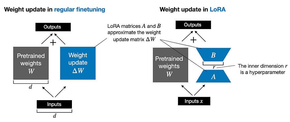
Low Rank Adaptation (LoRA): Aurora employs LoRA, a technique that allows for efficient fine-tuning of large models. Here’s how it works:
Instead of updating all model parameters, LoRA introduces small, trainable matrices to the attention layers.
For each linear transformation W in the self-attention layers, LoRA learns low-rank matrices A and B.
The output is computed as: Wx + BAx, where x is the input.
LoRA significantly reduces the number of trainable parameters, making fine-tuning more memory-efficient. LoRA for foundation models also comes with some other benefits-
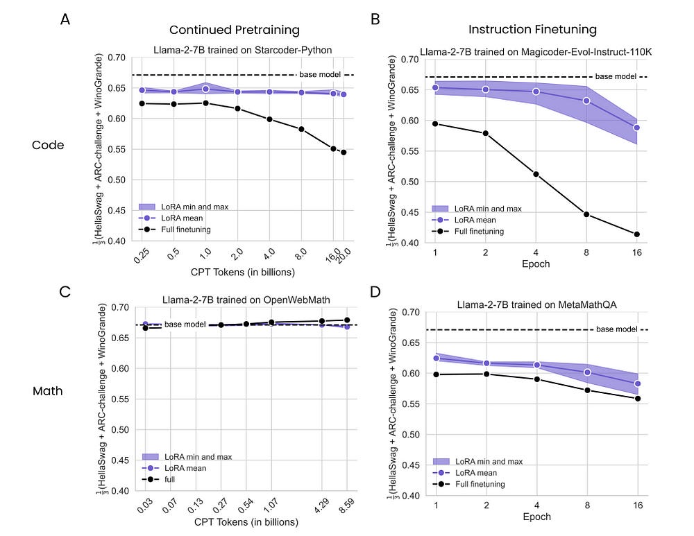
… LoRA saves memory by training only low rank perturbations to selected weight matrices. …Our results show that, in most settings, LoRA substantially underperforms full finetuning. Nevertheless, LoRA exhibits a desirable form of regularization: it better maintains the base model’s performance on tasks outside the target domain. We show that LoRA provides stronger regularization compared to common techniques such as weight decay and dropout; it also helps maintain more diverse generations….
-LoRA Learns Less and Forgets Less. Makes sense when you think about how LoRA will not rewrite as much of the params. The learning less is an acceptable tradeoff when you think that FT is not great for knowledge injection to begin with.
There is of course the forgetting less part, which is also helpful for us-
Pushforward Trick: To manage the computational complexity of backpropagating through long sequences, Aurora uses the “pushforward trick”:
Gradients are only propagated through the last roll-out step.
This approximates full backpropagation while dramatically reducing memory requirements.
This enables training on longer sequences without excessive memory usage.
Replay Buffer: Aurora implements a replay buffer, a technique borrowed from reinforcement learning:
A buffer stores a mix of initial conditions and model-generated predictions.
During training, samples are drawn from this buffer rather than always starting from true initial conditions.
This allows the model to learn from its own predictions, improving long-term stability and mimics the real-world scenario where forecasts are often made based on previous predictions rather than always starting from fresh observations.
By combining techniques from deep learning, reinforcement learning, and domain-specific insights, the authors have created a fine-tuning process that allows Aurora to excel at both short-term and long-term predictions. This approach not only pushes the boundaries of AI-based weather forecasting but also provides a framework that could be adapted to other domains requiring long-term sequence prediction.
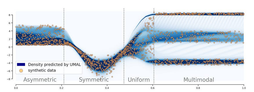
One way this could be upgraded is to rely on more probabilistic ensembles to model multiple behaviors. This is something Google’s Flood Forecasting System did really well, using an ensemble of Asymmetric Laplacians to model across the various ways the flood could play out. The use of an ensemble allowed different models to get different kinds of distributions, allowing them to capture relationships that were too complex for one architecture. But overall, this paper is super cool contribution that deserves a lot more attention than it has been given.
If this research interests you- I strongly suggest reading the original paper yourself. It’s important in this case for two reasons-
I’ve never taken a course in Machine Learning or Advanced Math, so there’s always a chance I misunderstood something (especially b/c scientists have this annoying tendency to reuse symbols across fields). I don’t think I have gotten anything wrong or overlooked the important ideas, but this is a big, complex publication, and it’s always good to verify for yourself.
You might find something very interesting and useful in something that I missed (in that case share it with me).
We will end this article here. I’ve already spent 12 hours on this, and my thinking is fried. I’m going to run hill sprints till I almost throw up to feel normal again.
If you liked this article and wish to share it, please refer to the following guidelines.
That is it for this piece. I appreciate your time. As always, if you’re interested in working with me or checking out my other work, my links will be at the end of this email/post. And if you found value in this write-up, I would appreciate you sharing it with more people. It is word-of-mouth referrals like yours that help me grow. You can share your testimonials over here.
Reach out to me
Use the links below to check out my other content, learn more about tutoring, reach out to me about projects, or just to say hi.
Small Snippets about Tech, AI and Machine Learning over here
AI Newsletter- https://artificialintelligencemadesimple.substack.com/
My grandma’s favorite Tech Newsletter- https://codinginterviewsmadesimple.substack.com/
Check out my other articles on Medium. : https://rb.gy/zn1aiu
My YouTube: https://rb.gy/88iwdd
Reach out to me on LinkedIn. Let’s connect: https://rb.gy/m5ok2y
My Instagram: https://rb.gy/gmvuy9
My Twitter: https://twitter.com/Machine01776819




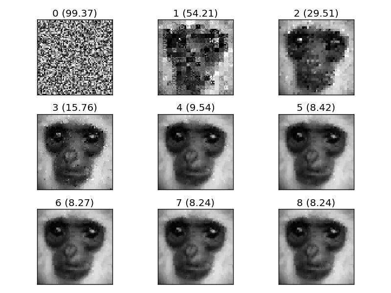



This does look similar to diffusion with all the level granularity.
Diffusion on weather really cool 🖤
Thank you for the breakdown! This is such an excellent use case for ML and I didn't even know about it until you sent out this article.